On writing clean Jupyter notebooks

Notebooks are a magnificent tool to explore data, but such a powerful tool can become hard to manage quickly. Ironically, the ability to interact with our data rapidly (modify code cells, run, and repeat) is the exact reason why a notebook may become an obscure entanglement of variables that are hard to understand, even to the notebook’s author. But it doesn’t have to be that way. This post summarizes my learnings over the past few years on writing clean notebooks.

I learned Python and discovered Jupyter notebooks about the same time, six years ago. The one thing that surprised me the most was how people could write code that others could reliably use. I looked upon projects like scikit-learn, which inspired me to start my first open source project. Fast forward, I learned a lot of software engineering practices like modularization and packaging. Still, I was unsure how to translate that to my data science work since data analysis comes with much more uncertainty and dynamism. But as the Python data tools ecosystem matured, I started to figure out how to make this work.

Summary

Here’s the breakdown:

1. Lock dependencies
2. Package your project
3. Modularize code
4. Be careful with mutable data structures
5. Auto-reload code from external modules
6. Unit testing
7. Organize in sections
8. Use a code linter
9. Use a code auto-formatter
10. Write shorter notebooks

Continue reading for details on each section.

Example code available here.

1. Lock dependencies

Before talking about clean notebooks, let’s spend some time talking about dependency management. Countless times, I’ve tried to execute an old notebook (from myself or someone else) and bump into multiple ModuleNotFound errors. Even after running pip install for each of them, it’s not uncommon to run into cryptic errors because the package API changed and is no longer compatible with the code.

To prevent broken notebooks due to missing dependencies. Each third-party package we use must be registered in a requirements.txt file (or environment.yml if we are using conda). For example, a typical requirements.txt may look like this:

matplotlib
pandas
scikit-learn

After installing our dependencies in a virtual environment (always use virtual environments!), we can generate an exhaustive list of all installed dependencies with:

pip freeze > requirements.lock.txt

And our requirements.lock.txt would look like this:

# some packages...
matplotlib==3.4.2
# ...
pandas==1.2.4
# ...
scikit-learn==0.24.2
# ...

Why does requirements.lock.txt contain so many lines? Each package has a set of dependencies (e.g., pandas requires NumPy); hence, pip freeze generates the list of all necessary packages to run our project. Each line also includes the specific installed version. Therefore, if we want to run our notebook one year from now, we won’t run into compatibility issues since we’ll install the same version we used during development.

Even if our project contains multiple notebooks, a single requirements.txt suffices. However, bear in mind that the more dependencies our project has, the greater the chance of running into dependency conflicts (e.g., imagine pandas requires NumPy version 1.1, but scikit-learn requires NumPy version 1.2).

Remember to keep your requirements.txt and ``requirements.lock.txt` up-to-date: add new packages if you need them and remove them if you don’t need them anymore.

2. Package your project

When writing a notebook, it’s tempting to start defining functions or classes in our notebook file, but this creates a few complications. First, it makes it impossible to import such code in another notebook, and second, it makes it hard to reason about its semantics (is this a function that processes data or plots it?). A better practice is to keep our function and class definitions in a separate file and import them in our notebook:

# plotting functions go here
plot.py
# processing functions go here
process.py
# exploration notebook
exploration.ipynb

Such a simple layout works fine until we want to organize our code in folders:

src/
    plot.py
    process.py
notebooks/
    exploration.ipynb

If we open exploration.ipynb, we can no longer do import plot or import process. That’s because when using import, Python first looks for a local module (i.e., file in the same directory) with that name, and then, it looks in site-packages (that’s where packages are stored when you do pip install {package}). Hence, if we want Python to import our code, we have to tell Python where to look for it. I’m sure you’ve seen this before:

import sys
sys.path.append('../src')

We are telling Python to look inside ../src for modules. If we do so, we’ll be able to import plot.py, and process.py. But this is a terrible practice. Modifying sys.path makes our code easy to break since it assumes the code we want to import exists in a specific location. If we move any of the .py files, we’ll break our notebook. Fortunately, there is a robust way to solve this problem: create a Python package.

A Python package is a collection of Python files that you can install with pip install {package}. pip takes care of configuring Python so that it knows where to look for the code. Creating a package is simple; it only requires you to add a setup.py file:

from glob import glob
from os.path import basename, splitext
from setuptools import find_packages, setup

setup(
    name='my_package',
    version='0.1',
    packages=find_packages(where='src'),
    package_dir={'': 'src'},
    py_modules=[splitext(basename(path))[0] for path in glob('src/*.py')],
)

Then, we make a small change to our project layout and put our code under a my_package/ directory and add an __init__.py file:

src/
    my_package/
        __init__.py
        plot.py
        process.py
notebooks/
    exploration.ipynb
setup.py

That’s it! If you move to the folder containing the setup.py file, you can do:

pip install --editable .

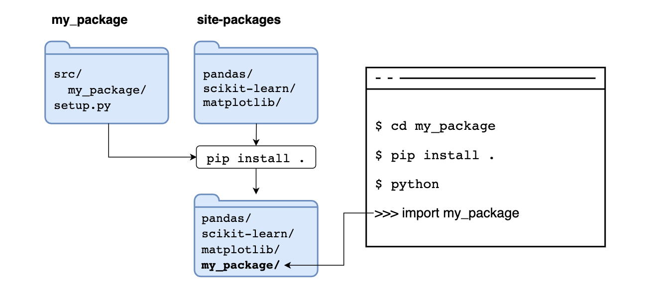
Let’s see what’s going on with this command. When installing a package via pip install {package}, we are telling pip to go to the Python Package Index, search for a package with the requested name, and store it in site-packages.

But pip can install from other locations. For example, suppose we execute pip install .. In that case, we are telling pip to use the source in the current directory, running such command copies the code and stores it in site-packages next to any other third-party packages, if we import it, it will read the copy in site-packages:

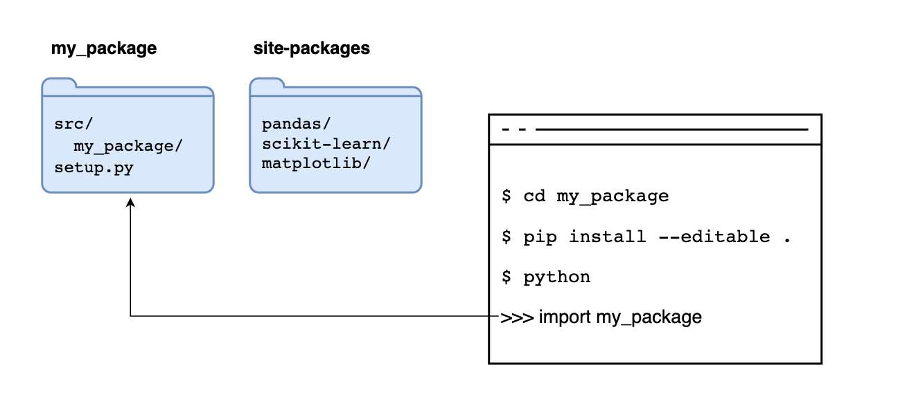
If we add the --editable flag, we tell pip not to copy the code but to read the code its original location, allowing us to make changes to our code and have Python use the latest version when importing it:

After installing our package, any module in the src/my_package/ folder is importable from any directory:

# all of these work regardless of the current working directory!
import my_package
from my_package import plot
from my_package.plot import some_plotting_function

There we go, no more sys.path fiddling!

3. Modularize code

When exploring data, most of the code looks like this:

# pandas operation
# another pandas operation
# some matplotlib call
# repeats...

But from time to time, there are pieces of code that have more structure:

1. Snippets that you call more than once
2. Snippets with control structures (i.e., if, for)

For the first kind, it’s best to abstract them into functions, and call them in your notebook. The second kind is a bit more subjective, and it depends on how complex the snippet is. If it’s a single control structure with a few lines of code in its body, it’s ok to leave it in the notebook, but if it’s more than one control structure with many lines in its body, it’s best to create a function, even if you’re using it only once, then call it in your notebook.

A clean notebook is effectively a series of lines of code with few to no structures of control. Sofware complexity formalizes in a metric called cyclomatic complexity that measures how complex a program is. Intuitively speaking, the more branches a program has (e.g., if statements), the more complicated it is.

Measuring notebooks complexity on each git push is a way to prevent overly complex notebooks from getting into the codebase, the mccabe package can measure cyclomatic complexity of Python programs:

jupyter nbconvert exploration.ipynb --to python
python -m mccabe --min 3 exploration.py

In the previous command, we’re only reporting parts of the notebook with a complexity of 3 or higher; this allows simple control structures to exist:

# these have a complexity of 2

if something:
    print('something happened')

for value in values:
    print(value)

But anything more complex than this (such as a nested control structure), is flagged:

for value in values:
    if value % 2 == 0:
        print('something happened')

4. Be careful with mutable data structures

Most data structures used for data manipulation are mutable, meaning you can set some initial values and modify them later. Take a look at the following example:

import pandas as pd

df = pd.DataFrame({'zeros': [0, 0, 0]})

# mutate stucture
df['zeros'] = df['zeros'] + 1

df
#    zeros
# 0      1
# 1      1
# 2      1

As we can see in the previous example, we initialized a data frame with zeros but then modified the values. In such a short code snippet, it’s easy to see what’s happening: we know that after mutating the data frame, the zeros column contains ones.

However, this same pattern causes issues if mutations hide inside functions. Imagine you have the following notebook:

import pandas as pd

# function definition at the top of the notebook
def add_one(df):
    df['zeros'] = df['zeros'] + 1

# loading some data at the top of the notebook
df = pd.DataFrame({'zeros': [0, 0, 0]})

# more code...
# ...
# ...
# ...

# a few dozen cells below...
add_one(df)

df
#    zeros
# 0      1
# 1      1
# 2      1

In this example, a mutation happens inside a function; by the time you reach the cell that contains the mutation add_one(df), you may not even remember that add_one changes the zeros column and assume that df still contains zeros! Keeping track of mutations is even more complicated if the function definition exists in a different file.

Ther are two ways to prevent these types of issues. The first one is to use pure functions, which are functions that have no side-effects. Let’s re-write add_one to be a pure function:

def add_one(df):
    another = df.copy()
    another['zeros'] = another['zeros'] + 1
    return another

Instead of mutating the input data frame (df), we’re creating a new copy, mutating it and returning it:

df = pd.DataFrame({'zeros': [0, 0, 0]})

ones = add_one(df)

df
#    zeros
# 0      0
# 1      0
# 2      0

One caveat with this approach is that we waste too much memory because every time we apply a function to a data frame, we create a copy. Excessive data copying can quickly blow up memory usage. An alternative approach is to be explicit about our mutations and keep all transformations to a given column in a single place:

def add_one_to_column(values):
    return value + 1

df = pd.DataFrame({'zeros': [0, 0, 0]})

# keep all modifications to the 'zeros' column in a single cell
df['zeros'] = add_one_to_column(df['zeros'])
# ...
# ...

The previous example modifies the zeros column but in a different way: add_one_to_column takes a single column as an input and returns the mutated values. Mutation happens outside the function in an explicit way: df['zeros'] = add_one_to_column(df['zeros']). By looking at the code, we can see that we’re modifying the zeros column by applying the add_one_to_column function to it. If we had other transformations to the zeros column, we should keep them in the same cell, or even better, in the same function. This approach is more memory-efficient, but we have to be extremely careful to prevent bugs.

5. Auto-reload code from external modules

One thing you may have tried before is to import a function/class into a notebook, edit its source code and import it again. Unfortunately, such an approach doesn’t work. Python imports have a cache system; once you import something, importing it again doesn’t reload it from the source but uses the previously imported function/class. However, there is a simple way to enable module auto-reloading by adding the following code at the top of a notebook:

%load_ext autoreload
%autoreload 2

Since this isn’t a Python-native feature, it comes with a few quirks. If you want to learn more about the limitations of this approach, check out IPython’s documentation.

6. Unit testing

Given how fast data scientists have to move to get things done (i.e., improve model performance), it’s not a surprise that we often overlook testing. Still, once you get used to writing tests, it radically boosts your development speed.

For example, if you’re working on a function to clean a column in a data frame, you may interactively test a few inputs to check whether it is working correctly or not. After testing manually to ensure your code works, you move on. After some time, you may need to modify the original code to work under a new use case, run some manual testing and keep going. That manual testing process wastes too much time and opens the door to bugs if you don’t test all cases. It’s better to write those manual tests as unit tests so you can quickly run them on each code change.

Say you want to test your process.py; you can add a tests/test_process.py:

src/
    my_package/
        plot.py
        process.py
notebooks/
    exploration.ipynb
tests/
    test_process.py

And start writing your tests. I usually create one file in the tests/ directory for each file in the src/ directory with the name test_{module_name}.py. Such a naming rule allows me to know which test file to run when making changes to my code.

There are many frameworks for running tests, but I recommend you to use pytest. For example, suppose we are writing a function to clean a column that contains names, and we are using it in our notebook like this:

import pandas as pd
# Note that we're defining the function in a Python module, not in the notebook!
from my_package.process import clean_name

df = pd.DataFrame({'name': ['Hemingway, Ernest', 'virginia woolf',
                            'charles dickens   ']})

df['name'] = df.name.apply(clean_name)

After exploring the data a bit, we’ll find what kind of processing we must apply to clean the names: capitalize words, swap order if the name is in the “last name, first name” format, remove leading/trailing whitespace, etc. With such information, we can write (input, output) pairs to test our function:

import pytest
from my_package import process


@pytest.mark.parametrize(
    'name, expected',
    [
        ['Hemingway, Ernest', 'Ernest Hemingway'],
        ['virginia woolf', 'Virginia Woolf'],
        ['charles dickens   ', 'Charles Dickens'],
    ],
)
def test_clean_name(name, expected):
    # 1. Check process.clean_name('Hemingway, Ernest') == 'Ernest Hemingway'
    # 2. Check process.clean_name('virginia woolf') == 'Virginia Woolf'
    # 3. Check process.clean_name('charles dickens   ') == 'Charles Dickens'
    assert process.clean_name(name) == expected

Here we are using the @pytest.mark.parametrize decorator to parametrize a single test for each (name, expected) pair; we call our clean_name function with name and check if the output is equal to expected.

Then to run your tests:

pytest tests/

Writing tests isn’t trivial because it involves thinking of representative inputs and their appropriate outputs. Often, data processing code operates on complex data structures such as arrays or data frames. My recommendation is to test at the smallest data unit possible. In our example, our function operates at the value level; in other cases, you may be applying a transformation to an entire column, and in the most complex case, to a whole data frame.

Learning how to use the Python debugger is a great skill for fixing failing test cases. Suppose we’re working on fixing a test. We can rerun our tests, but this time stop execution whenever one of them fails:

pytest tests/ --pdb

Upon failure, an interactive debugging session starts, which we can use to debug our pipeline. To learn more about the Python debugger, read the documentation

Note that the previous command starts a debugging session at any given line that raises an error; if you want to start the debugger at an arbitrary code line, add the following line:

def some_function():
    # some code...

    # start debugger here
    from pdb import set_trace; set_trace()

    # more code....

And run your tests like this:

pytest tests/ -s

Once you’re done, remove from pdb import set_trace; set_trace() from your code.

If instead of the debugger, you want to start a regular Python session at any given line:

def some_function():
    # some code...

    # start python session here
    from IPython import embed; embed()

    # more code....

And invoke your tests the same way (pytest tests/ -s)

7. Organize in sections

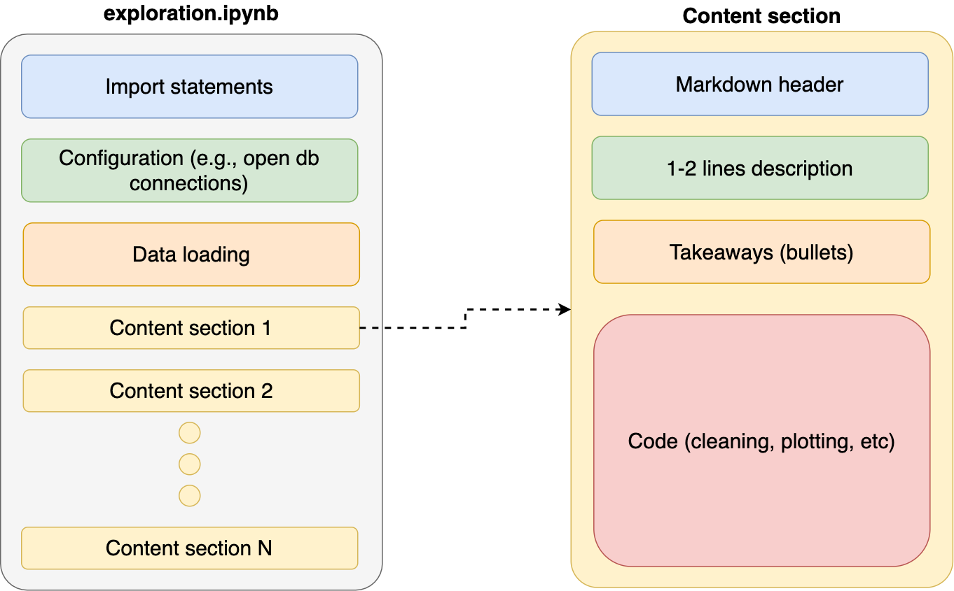
When exploring data, it’s natural to write code organically as we learn more about our it; however, it’s important to revisit our code and re-organize it after achieving any small goal (e.g., creating a new chart). Providing clear organization to our notebooks makes them easier to understand. As a general rule, I keep my notebooks with the same structure:

1. Import statements
2. Configuration (e.g., open database connections)
3. Data loading
4. Content

With each content section having a standard structure:

1. Markdown header (e.g., # My notebook section)
2. Description. One or two lines summarizing what this section is about
3. Takeaways. A few bullets with the most important learnings of this section
4. Code. Actual program that cleans, analyzes, or plots data.

8. Use a code linter

When refactoring old code, we may overlook cleaning it up thoroughly. For example, suppose we were using a package called some_plotting_package to create some custom charts but find out it is not what we were looking for. We may delete the cells calling such a package but forget to remove the import some_plotting_package statement. As we write more extensive programs, it’s easy to overlook these small details. While they may not have any effect on the program’s execution, they’ll have a significant effect on readability.

Most text editors have plug-ings that detect issues and flag problematic lines. Here’s a screenshot of Visual Studio Code showing a problem in the first line (matplotlib is imported but unused):

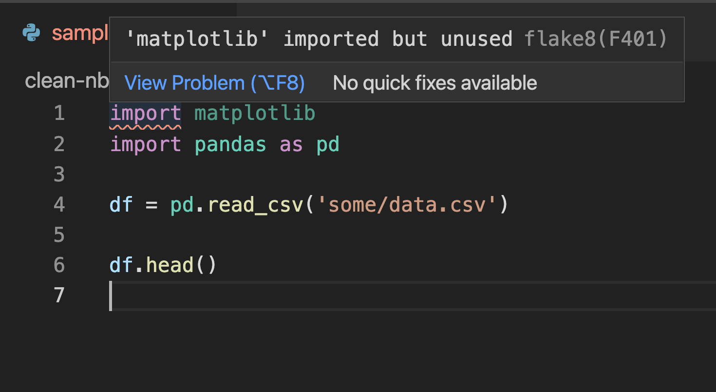
Unfortunately, there aren’t many linting plugins for Jupyter notebook/lab. The most reliable option seems to be jupyterlab-flake8, but the project seems abandoned.

The best way I’ve found to lint my notebooks is not to use .ipynb files but vanilla .py ones. jupytext implements a Jupyter plugin allowing you to open .py files as notebooks. For example, say you have an exploratory.ipynb, and you want to start linting it. First, convert the notebook to a script using jupytext:

jupytext exploration.ipynb --to py

The command above generates an exploratory.py that you can still open like a notebook. If using jupyter notebook, this happens automatically; if using jupyter lab, you need to Right Click -> Open With... -> Notebook.

After editing your “notebook”, you can open it in any text editor that supports Python linting; I recommend Visual Studio Code since it’s free and pretty easy to set up for Python linting. Note that there are many options to choose from; my recommendation is to use flake8.

Note that since .py files do not support storing the output in the same file, all tables/charts delete if you close the file. However, you can use jupytext’s pairing feature to pair a .py file with a .ipynb one. You edit the .py file, but the .ipynb notebook serves to back up your output.

9. Use a code auto-formatter

Linters only indicate where problems are but do not fix them; however, auto-formatters do that for you, making your code more legible. The most widely used auto-formatter is black, but there are other options such as yapf.

Ther are a few options to auto-format .ipynb files (one, two, three). I haven’t tried any of these, so I cannot comment on their usage. My recommended approach is the same described in the previous section: use jupytext to open .py files as notebooks, then apply auto-formatting to those .py files using Visual Studio Code. Click here for instructions on setting up formatting in VS Code.

Note that auto-formatters do not fix all the problems linted by flake8, so you may still need to do some manual editing.

10. Write shorter notebooks

Since notebooks are written interactively, we tend to use short variable names, often following conventions dictated by the libraries we’re using. More times than I’m willing to admit I’ve made the mistake of doing something like this:

import pandas as pd

df = pd.read_csv('/path/to/data.csv')

# 100 cells below...

df = pd.read_csv('/path/to/another.csv')

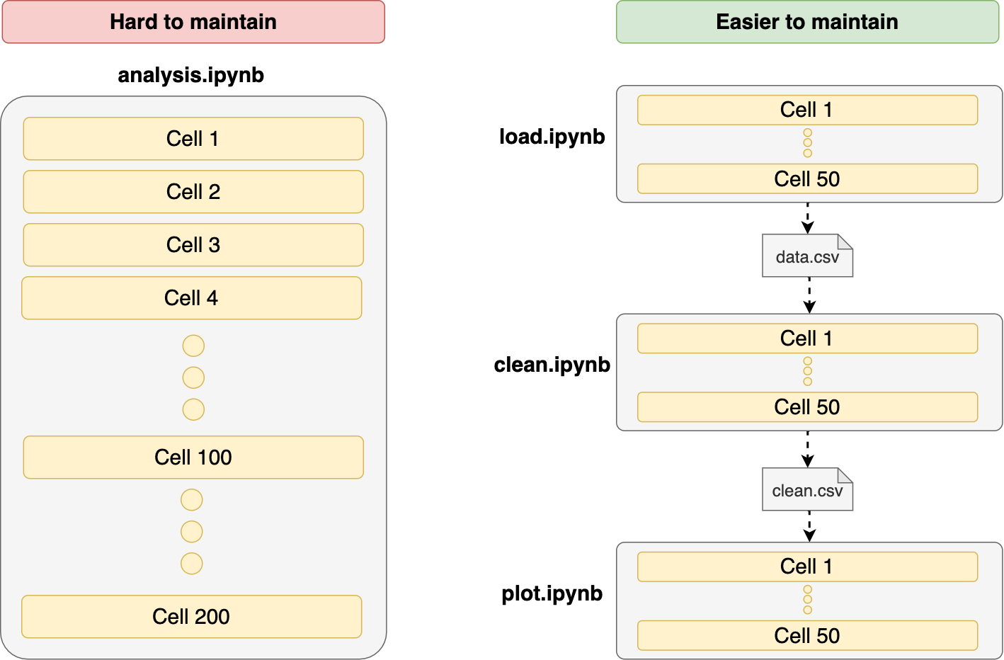
Re-using variable names is a significant source of errors. When developing interactively, we may want to save some keystrokes and assign short names to most variables. That’s fine for getting a rapid exploration experience, but the longer our notebooks are, the higher the chance of running into these issues. The best approach is to break our notebooks into smaller parts to reduce the possibility of side effects.

Breaking down notebooks in multiple parts isn’t as easy as it sounds because we have to find ones to connect one piece to the next one (i.e., save our data frame and load it in the next one), but doing it will help us create more maintainable code.

How to decide when it’s ok to add a new cell and when to create a new notebook it’s highly subjective, but here are my rules of thumb:

1. Different datasets must be in a different notebook
2. When joining datasets, create a new one
3. One notebook for data cleaning, another one for plotting (or feature generation if doing ML)

Of course, this depends on the complexity of your project. If you’re working with a small dataset, it may make sense to keep everything in a single notebook, but as soon as you’re working with two or more sources of data, it’s best to split.

If you want to save time concatenating multiple notebooks into a single coherent analysis pipeline, give Ploomber a try. It allows you to do just that and comes with a lot more features such as notebook parallelization, debugging tools, and execution in the cloud.

Final thoughts

Writing clean notebooks takes some effort, but it’s definitely worth the price. The main challenge with writing clean code is to achieve a healthy balance between iteration speed and code quality. We should aim to set a minimum level of quality in our code and improve it continuously. By following these ten recommendations, you’ll be able to write cleaner notebooks that are easier to test and maintain.

Do you have other ideas on improving the Jupyter notebook’s code quality? Please reach out. I’m always excited to discuss these topics.

Thanks to Filip Jankovic for providing feedback on an earlier version of this post.