Causal Inference and Experimentation in Python - Part I

Hello everyone, this is Harrison from Ploomber! I am writing a three-part series detailing causal inference in data science utilizing Ploomber and PyMC. Specifically, Part One will discuss causal inference in data science, designing experiments in the absence of ideal A/B test conditions, and inference (I will use inference interchangeably with causal inference throughout) via Regression Discontinuity Designs (RDDs). RDDs are a special natural experiment framework for analyzing causal relationships. Deducing causal relationships at scale is difficult, but I will outline potential methodologies to create experiments that overcome these difficulties. Parts Two and Three will showcase a practical RDD testing pipeline utilizing Ploomber and discuss Ploomber’s value-add in large-scale causal inference testing. Enjoy!

I. Causal Inference in Data Science

Causal inference and prediction tasks are distinct tasks. Unfortunately, their methods are often conflated within an analytics pipeline. What does each task accomplish? How can we leverage a task’s unique outcomes?

Prediction vs Inference

Here’s a pleasant, metaphorical representation of the divergence in causal inference and prediction tasks. Credit to Jens Lelie on Unsplash.

An overwhelming majority of work in Data Science/Machine Learning (DS/ML) revolves around solving prediction problems. To illustrate this point, I will list a few problems I’ve tackled during data science recruiting alone (not breaking any NDAs here): predicting customer churn rates with time series data; predicting hotel price changes based on a user’s socioeconomic characteristics; predicting customer sentiment through product review text data. You get the point - we are modeling some target measure (churn, price, sentiment, etc. ) as a function of some sample of relevant features.

Prediction tasks are and continue to be the focus of modeling efforts throughout the industry, but firms have started to invest significant resources in causal inference pipelines. Firms are experimenting with models that (attempt) to link factors (features, variables, covariates, all that jargon) with change in a target’s prediction. This sounds a lot like A/B testing!

You’d be right to assume that A/B testing is a branch of inference. We are trying to find how change in A affects change in B. However, and I emphasize this point, the statistical methodologies and experimental designs underlying A/B testing are less rigorous compared to causal inference pipelines. Don’t believe me? Consider companies like Uber, Microsoft, and IBM, who maintain growing open source python packages dedicated to inference/causality modeling.

It’s natural to view the activities of monolithic tech companies with guarded skepticism, but it’s worth acknowledging that a greater number of business problems are now addressed via causal inference frameworks. Perhaps its being used to develop KPI’s for products; maybe its for gauging business health. Either way, adoption is slowly growing amongst practitioners. In other words, reader who is a member of the DS/ML industry, it is critical for you to:

• assess how potential industry trends affect the scope of a data scientist’s role AND

• ascertain the appropriate tools/workflows that maximize a data scientist’s productivity in accordance with these trends

Although data scientists are increasingly adopting casual methodologies to diagnose and explain business issues, it’s essential to understand why causal ML methods have had limited use up until this point.

Inference questions are difficult to test due to data complexity and randomness throughout the modeling process. When compared to prediction tasks, structural limitations imposed by big data collection and modeling algorithms can generate conflicting results. Say we generate two models (predictive and inferential) that utilize the same features and target variable. Here, modeling discrepancies lie in the varying influences of our covariates; certain features may appear unimportant when solving the prediction task, but may play important roles estimating treatment effects for an inference task. Other technical obstacles, specifically difficulties scaling to large datasets, impede the viability of causal inference analyses. There are many technical barriers for inference at scale I will not cover in this post, but it is important to understand that an experiment’s design can overcome these barriers. Designing an appropriate experiment, as with every other step in the DS/ML pipeline, requires some finesse.

Wait, What is Causal Inference Again?

I’ll continue adding funny quips under these abstract stock photos. We’re looking to directly connect change in some variable to our target. Credit to Bruno Figueiredo on Unsplash

Right, we never talked about the distinction between prediction and causal inference tasks. Let’s take a step back.

Often, prediction and inference tasks are completed in tandem -  we make assumptions about deducing the structure of our data-generating process (inference) while using these assumptions to guess the output of future data (prediction). It is important to recognize that:

• prediction and inference tasks are distinct procedures, generating different outcomes

• the procedures necessitate unique methodological considerations

• outcome discrepancies and methodological considerations lead to distinctive insights and applications for the practitioner

The third point is the most salient for the purposes of this article. It is erroneous to claim that prediction or inference tasks are more useful (as a whole) to the data scientist. Situationally, however, it may be more appropriate/practical to exploit the respective outcomes of each task.

NOTE: this post is not a teleological argument for causal inference, just a brief primer on its methods and takeaways.

I mentioned previously that covariate importances/interpretations may differ depending on the task that one is accomplishing. As is the case in ML, there is a tradeoff associated with the model predicting effectively, and the model accurately characterizing the data generating process. In other words, there is an important tradeoff between the accuracy and interpretability of a ML model. For causal inference, there is an emphasis on increasing model interpretability. This emphasis allots causal inference and its experimental designs two great strengths: affecting policy to change some desired outcome and measuring change from this policy (jargon alert: I will use policy, treatment, and intervention interchangeably to describe the process of enacting change on a group of observations during an experiment).

Specifically, when we enact some policy we can:

• design tests to measure changes between a pre and post-intervention setting

• evaluate whether our intervention resulted in statistically significant or random change

To restate, causal inference connects change in specific covariates to change in a desired target. If this change is statistically significant, organizations can make actionable decisions to achieve a desired outcome.

NOTE: metrics to evaluate one policy’s efficacy over another are not covered in this post. You could do it numerically, but this necessitates additional testing frameworks that I will not talk about.

Although predictive models are more accurate and scalable than inference methods, inference’s connection between policy and change can be leveraged in distinct manners. Specifically, inference’s conclusions can generalize to wider contexts (compared to prediction models) depending on an inference experiment’s internal and external rigor. Thus, measuring change via causal frameworks yields a more deliberate approach to ML model construction.

In sum, prediction and inference tasks are often conflated during the insight-generation process. Procedures from both tasks are combined to produce a desired result. Inference is concerned with validating the contributions of individual variables in a model. Specifically, gauging the variable’s ‘importance’ for inducing change - contingent on its underlying statistical properties (more on this later). The key distinctions between prediction and inference can be thought of in terms of specificity and scope for variables. During prediction, the underlying statistical validity of variables is not investigated. In addition, although the magnitudes of individual coefficients are given in prediction tasks, individual coefficients are aggregated in a single measure. For supervised problems (we have a predicted measure and base truth for this prediction), these predicted aggregates measures are compared against their respective base truths. There are many more distinctions, but these provide a basis for determining causality.

II. Causal Inference via RDD

We’ve learned a few of the distinctions between prediction and inference. So - what are the designs of causal inference frameworks?

A/B Testing and its Limitations

In industry, A/B testing is widely used to approximate causal relationships. Although experimental design varies widely, ideally we want to replicate randomized controlled trial (RCT) methodologies to the best of our ability. This is where things get dicey - in some situations ideal conditions for randomized controlled trials cannot be achieved. Oftentimes, researchers cannot assign treatment at random due to practical or ethical considerations. The canonical example of bad ethics (something I was taught as an economics undergraduate) would be a large-scale RCT forcing child participants to smoke real/placebo cigarettes (treatment and control, respectively) throughout adulthood to measure the effects of smoking on adolescent health.

It’s comically extreme, but the example does illustrate that practical considerations must be made when investigators implement a causal inference model. When RCT conditions cannot be upheld, alternative methodologies for experimentation must be adopted. One of these alternatives is a family of tests classified as natural experiments.

Natural Experiments

No more silly captions after this one. Let’s use forces out of our control to run valid experiments. Photo by Ivan Bandura on Unsplash

Natural experiments are pseudo-randomized observational studies that we can use to derive causation. The idea is as follows: natural forces (time, geography, any force that cannot be controlled by a researcher) affecting the outcomes of an observational study emulates the randomness conditions of a RCT. The natural forces that affect experimental outcomes tend to vary, but the key here is that the unit of comparison (people, geographic regions, etc.) can be easily distinguished as treated or not treated.

Now you may be thinking, if the groups are easily distinguishable between treatment and control, then how can we closely match RCT conditions? The key here is that assignment to the control is randomized by the natural force. So, to reiterate, natural forces randomly assign participants to treatment and control groups (think of this as a policy that is implemented at random). We can harness the force’s unexpected introduction and the resulting control/treatment division to measure changes for some shared quality. As data scientists, we can create natural experiment conditions by:

• finding the right randomizing “force” that acts upon a specific independent variable AND

• easily distinguishes the control/treatment groups (binary outcome) in order to

• extract causal relationships

Natural Experiments - An Example

A (semi-famous/canonical) natural experimentation setup: we are studying the relationship between alcohol consumption and mortality rates. Specifically, we are analyzing whether alcohol consumption just above and below the drinking age increases mortality rates. To test this, we utilize changes in state drinking laws throughout the 1970s and 1980s (the random force) to study if there are differences in mortality rates amongst adults barely-over and barely-under the new minimum legal drinking age (control/treatment groups based on MLDA).

We obtain data on alcohol-related fatalities by state and survey data on alcohol consumption for 19-23 year old adults. We validate underlying normality assumptions for linear regression (our data is i.i.d., there is no variation in our error terms, etc.) and split our observations into appropriate, comparable groups. Then, we graph trends plotting age against drinking behavior for our appropriate groups, observing if there is a distance between mortality rates at the 21 year cutoff we’ve described (extract causal relationships between drinking and mortality rates).

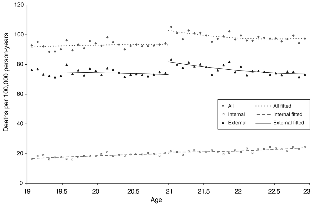
Regression Discontinuity comparing Age Profiles and Death Rates. The figure plots alcohol related mortality rates for young adults ages 19-23. Reprinted with permission from NIH National Library of Medicine’s in Author Manuscripts. “The Effect of Alcohol Consumption on Mortality: Regression Discontinuity Evidence from the Minimum Drinking Age,” by C. Carpenter and C. Dobkin, 2009, American Journal of Applied Economics, 1(1), 164-182.

As you can see, there is a sharp increase in mortality rates after the MLDA threshold! Our work, however, is not over. We must address outside influences on drinking behavior to have externally valid results. What do I mean by the latter? After properly validating internal modeling assumptions with appropriate statistical considerations (many times, this can be done via the central limit theorem and the law of large numbers), we must consider outside causes that may affect the relationship between drinking and mortality. For example, is the increase in mortality due to people who just started experimenting with drinking (new drinkers)? Furthermore, is this increase in mortality from existing alcohol users who began experimenting with binge drinking (existing drinkers increasing their consumption)?

If we utilize other variables from our datasets, we can plot these potential confounding relationships and show that there is no evidence to support these claims (I won’t go into extensive detail in the post, but the results can be found in the discussion section of this paper). Rushed reasoning aside, the important takeaways here are that:

• we should be mindful about potential outside (exogenous) forces that could affect our model AND

• implement research designs that could explain away/minimize the impact of these forces 

If we can protect our analysis from these external “threats” through a number of broad, logical assertions (these come from intentional research design), we can design causal inference models under natural experiment conditions. It’s an art, not a science.

If you are interested in learning more about natural experiment setups, here is another famous paper that contextualizes research design decisions.

III. Regression Discontinuity Designs

Okay, we’ve learned about natural experiments. With all of this out of the way, we can talk about Regression Discontinuity Design (RDD)! Specifically, I will be talking about Sharp RDDs throughout this post, using RDD as an abbreviation. There are alternative discontinuity designs (Fuzzy RDDs to be specific) that are not within the scope of this post, but have useful implementations under certain conditions. Distinguishing characteristics of Sharp and Fuzzy RDDs are briefly mentioned below.

An Overview: Visualizing Sharp RDD

I explain the components of the RDD at a high level overview before I detail implementation specifics.

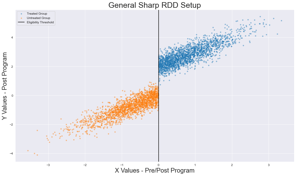
1. a threshold (the black line) is determined; it divides subjects between control and treatment groups
2. we plot two linear regressions, one for each group’s distribution (orange and blue, respectively)
3. at the previously determined threshold, we map the difference between the plotted regressions
4. a battery of tests are then conducted to determine the validity of the difference

In sum, two regressions are constructed on opposite sides of a threshold (an arbitrary value from a continuous variable). At the threshold, the distance between these two regressions is calculated and then analyzed to determine statistical significance. We leverage the intuitions

1. that points around this regression tend to share similar characteristics AND
2. the arbitrariness of our threshold allots to sufficient randomization of our two groups

With these two qualities, we can measure a our change based on similarities. You may be thinking: How does this relate to natural experiments? How do we determine the validity of our results? The specifics follow.

Regression Discontinuity - The Specifics

The evaluation of a successful RDD involves several steps:

Selecting a running variable. The running variable (RV) has several names (eligibility variable, selection variable), but I will refer to it as a RV henceforth. The RV is a continuous variable that determines eligibility for treatment. Think of it as the variable that makes up the x-axis of a 2D graph. Here, there are two main points to emphasize. First, the variable must be continuous (for reasons that will become apparent). Second, the variable must determine treatment eligibility. Remember how I said that natural experiments must have a way to easily sort people between treatment and control groups? The RV is the basis for delineating between those two groups. The way we sort the two groups is by….

Identifying an eligibility threshold. The eligibility threshold is an arbitrary RV value that separates the treatment and control groups. In essence, the eligibility threshold is a line that determines treatment/control assignment: values on one side of the line are all labeled as treated while all values on the other side are labeled control. I refrain from using cardinal directions (all values on the right/left side of the line are labeled as *insert group designation*) because research design can vary. For example, say a study has observations whose RV takes on values between 0 and 200. Say that the eligibility threshold is assigned at 100. Researchers may decide to assign all values above 100 to the treatment group and all values below 100 to the control group. The opposite situation is just as plausible: all values below the threshold are assigned to the treatment group and all values above the threshold are assigned to the control group. In both situations, assignment to treatment or control groups is absolute.

NOTE: There is an RDD method that accounts for cases where assignment is not absolute after an eligibility threshold is determined, (i.e. some values within the control group may be treated and vice versa). I do not cover this method in this post, but feel free to check out this resource on fuzzy regression discontinuity

Plotting Regressions over Group Distributions. After we assign membership to our observations based on the threshold, we can plot regressions over the treatment and control distributions. Although many studies utilize linear regressions to map these distributions, polynomial regressions are perfectly acceptable should they fit the data better. 

Measuring Treatment Effects. If a discrepancy exists between regressions, we can measure the distance between the regressions at the threshold to measure the treatment effect’s size and sign. Here the discrepancy/discontinuity in our plotted regressions is a result of a policy intervention, implying that the regressions themselves are being plotted on data after the event of this intervention. This is absolutely critical in understanding the power of RDDs. We assume that, ceteris paribus, the policy is the only reason for the shift in the RV’s relationship with the target variable. 

The data following the policy implementation is part of the post-program distribution (this is the data we are plotting). The counterfactual (the unobserved alternative where the policy has not been implemented), is the pre-program distribution. For the counterfactual, we assume that the relationship between the RV and the target would be constant.

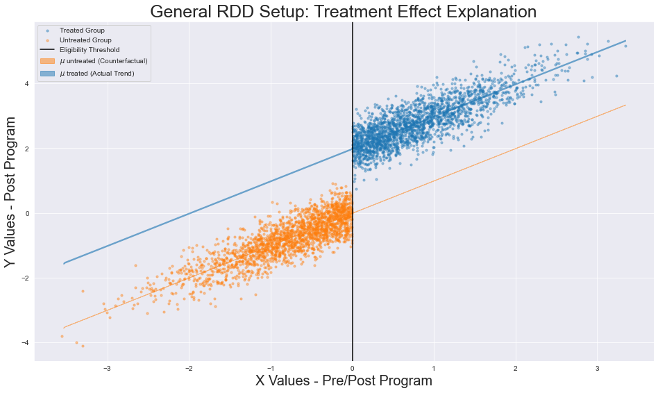
The difference in the true trend and the imagined counterfactual allows us to measure the size and magnitude of effect

In other words, the counterfactual assumes that in the event that the program had not been implemented, then a discontinuity would not exist at the eligibility threshold (the relationship between the RV and target would be continuous). By believing that, pre-program, a discontinuity would not exist, we can leverage the disparity between post-program treatment and control group regressions as evidence of change.

Now that we have a basis for evaluating the size of the difference, we need to understand whether policy generated positive or negative change. This is entirely situation-dependent. Above, I stated that experiment design can vary. Depending on the running variable, the target variable, and the location of the treatment/control groups, outcomes can change the interpretation of our results.

Positive Effect

Suppose that we are testing how customer satisfaction changes in accordance with the lateness of delivery. We assume that there is a constant inverse relationship between late delivery times and customer satisfaction. Say we decide to offer a refund to every customer past a certain point, let’s say 50 minutes:

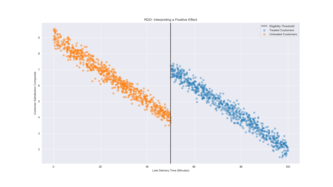
Here we show that the discontinuity has a positive effect - those who received a refund had higher (albeit diminishing) customer satisfaction levels despite the fact that their order was received later. 

Negative Effect

a hospital that monitors the health of its patients using some continuous measure. Suppose this hospital implements a new training program for doctors to lower the number of quality of care complaints they receive. We can assume that there is also an inverse relationship here between the health composite and the quality of care complaints. The hospital observes higher complaint rates for lower composite patients, so all doctors who have patients below a certain level receive this training.

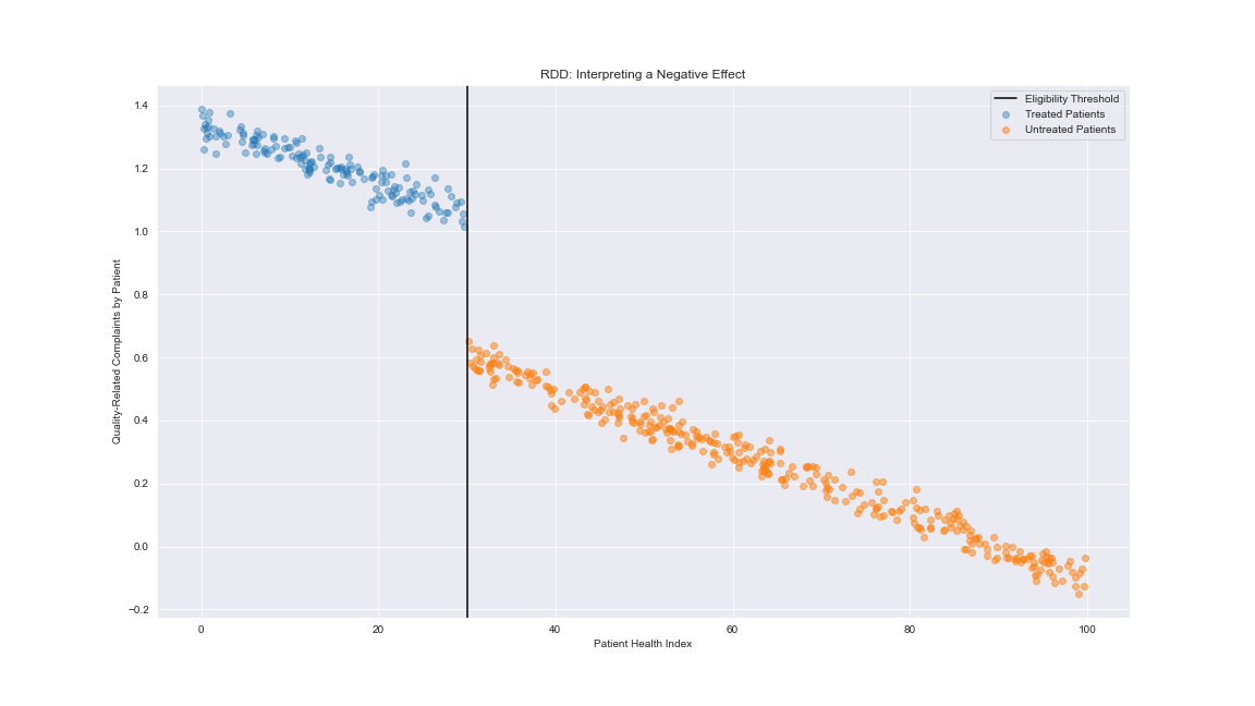
For some reason or another, the number of complaints increases despite additional training. This would result in a negative effect in the post-program group. Obviously, depending on the inputs of our experiment, there are significant differences in the inferences we draw. Practitioners should be mindful that the setup of the experiment (the RV, the threshold, the program, the target) can significantly impact the direction one takes with their subsequent analysis.

Model Diagnostics. Although we’ve determined the sign and magnitude of our treatment effect, we must determine the validity of these results. Without the model validation step, it may be the case that our results are the product of random chance. For regression discontinuity designs, we make two assumptions: model continuity and no sorting across the cutoff.

1. Model continuity assumes that (besides the RV you are testing/plotting) all covariates are continuous at the cutoff. This implies that the RV you are testing (post-program) is the only covariate with a discontinuity. This is relatively easy to diagnose - one can plot scatterplots of all other covariates with the target variable and assess whether discontinuities exist between the control and treatment groups. If there aren’t any observable differences between the other covariates and the target, then the threshold for eligibility chosen along the RV passes our first test. 
2. Assumption two, no sorting across the cutoff, is slightly more abstract. When running RDDs, we assume that observations in our study are not selecting their treatment status. To elaborate, observations around the treatment (whether it be directly above or below) are not “making decisions” that move them to either the treatment or control group. Take, for example, a government program that provides stipends to those with incomes below $50K. We assume that people who make $50.5K are not choosing to suppress their true income (perhaps they’re lying on their tax forms or asking their boss for a salary decrease) in order to qualify for the stipend. Regardless of the example’s context, we assume that observations are not intentionally manipulating their RV to acquire a certain treatment status. To validate assumption two, we can plot the empirical distribution of the running variable we are utilizing. Specifically, we are looking for clustering around the eligibility threshold of the distribution. If there is clustering, then there is reason to believe that sorting may be occurring. If the empirical distribution is (for the most part) smooth/lacks odd discontinuities, then there is not sufficient evidence for sorting behavior. 

Congratulations, you just survived a 3000+ word diatribe on causal inference in data science, A/B testing via natural experiments, and RDDs. To summarize, we covered the advantages of using causal inference as data scientists, instances where natural experiment designs must be considered, and a brief overview of the theory governing Sharp RDD. In parts two and three, I will cover how Ploomber-powered pipelines can parallelize causal inference in the cloud. I will walk through how I created a Bayesian RDD model in PyMC and outline how Ploomber can create modular pipelines for running experiments. For now, take some time to go outside and feel the sun’s warmth.