


Dash is a powerful framework for creating interactive, data-driven web applications, ideal for dynamic visualizations that transform raw data into actionable insights. A key feature of Dash apps is their ability to update graphs and other components based on user interactions such as selections from a dropdown, slider adjustments, or hovering over data points.
For scenarios requiring monitoring or receiving real-time data—such as tracking financial markets or IoT sensor streams—your components may need updates at regular intervals, from seconds to minutes. Today, we’ll focus on updating graphs based on a predefined interval.
There are two primary methods to update graphs in Dash:
This tutorial will concentrate on the second approach, demonstrating how to create graphs that smoothly update with new data arrivals, eliminating the need to redraw the entire plot. Follow along to build a real-time Bitcoin monitoring app using Dash and WebSocket API!
Our Bitcoin trade monitoring app consists of two main components:
Backend (Data Fetching and Storage): This component connects to the Binance WebSocket API to receive real-time trade data for Bitcoin (BTC/USDT). It processes the incoming data and stores it in a PostgreSQL database equipped with the TimescaleDB extension for efficient time-series data management. The backend functionality is implemented in websocket_backend.py.
Frontend (Real-time Monitoring Dashboard): This component establishes a Dash application to visualize the Bitcoin trade data stored in the database. It utilizes Dash’s dcc.Interval component to periodically fetch the latest data and update the graph. The frontend is implemented in app.py.
Given the need to fetch data asynchronously via the WebSocket API, separating the data fetching and visualization components is essential. This modularity ensures that the backend handles concurrent data fetching from the WebSocket API and database writing operations in TimescaleDB, while the frontend focuses on delivering a responsive user interface for real-time data display.
Before we dive deeper, let’s preview what our dashboard will look like:
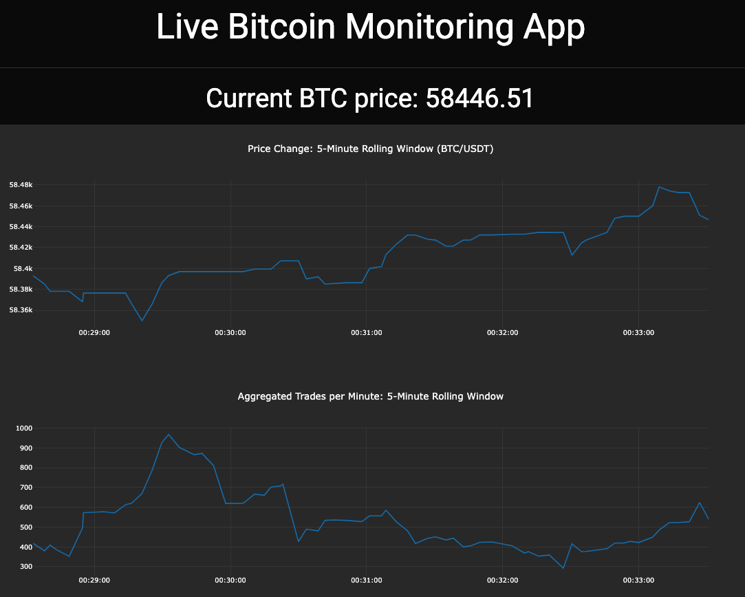
It has three main components:
Note: If you are primarily interested in the implementation of the Dash app and how to append new data to the existing graph, feel free to skip the backend part and proceed directly to the Frontend for a Real-time Monitoring App section.
Let’s set up your development environment to ensure that all necessary libraries are available and properly configured. Create a new virtual environment for this project with python, if you are using conda:
conda create --name YOUR_ENV_NAME python=3.11
conda activate YOUR_ENV_NAME
Create a requirements.txt file containing all the libraries needed for both the backend and frontend components of our application.
python-dotenv
dash
dash-bootstrap-components
psycopg2-binary
asyncpg
websockets
Then, run the following command to install the listed dependencies:
pip install -r requirements.txt
Now, we are ready to dive into it!
For this tutorial, we will utilize TimescaleDB, a PostgreSQL extension tailored for time-series data. It optimizes large dataset handling with features like automated data retention and continuous aggregation, maintaining performance while supporting full SQL for complex queries.
Note: Using TimescaleDB is not mandatory for this tutorial. TimescaleDB currently offers a 30-day free trial, so you can follow this tutorial using it, or adapt the steps for a local database like SQLite or another remote database. The coding approach will remain similar regardless of the database used.
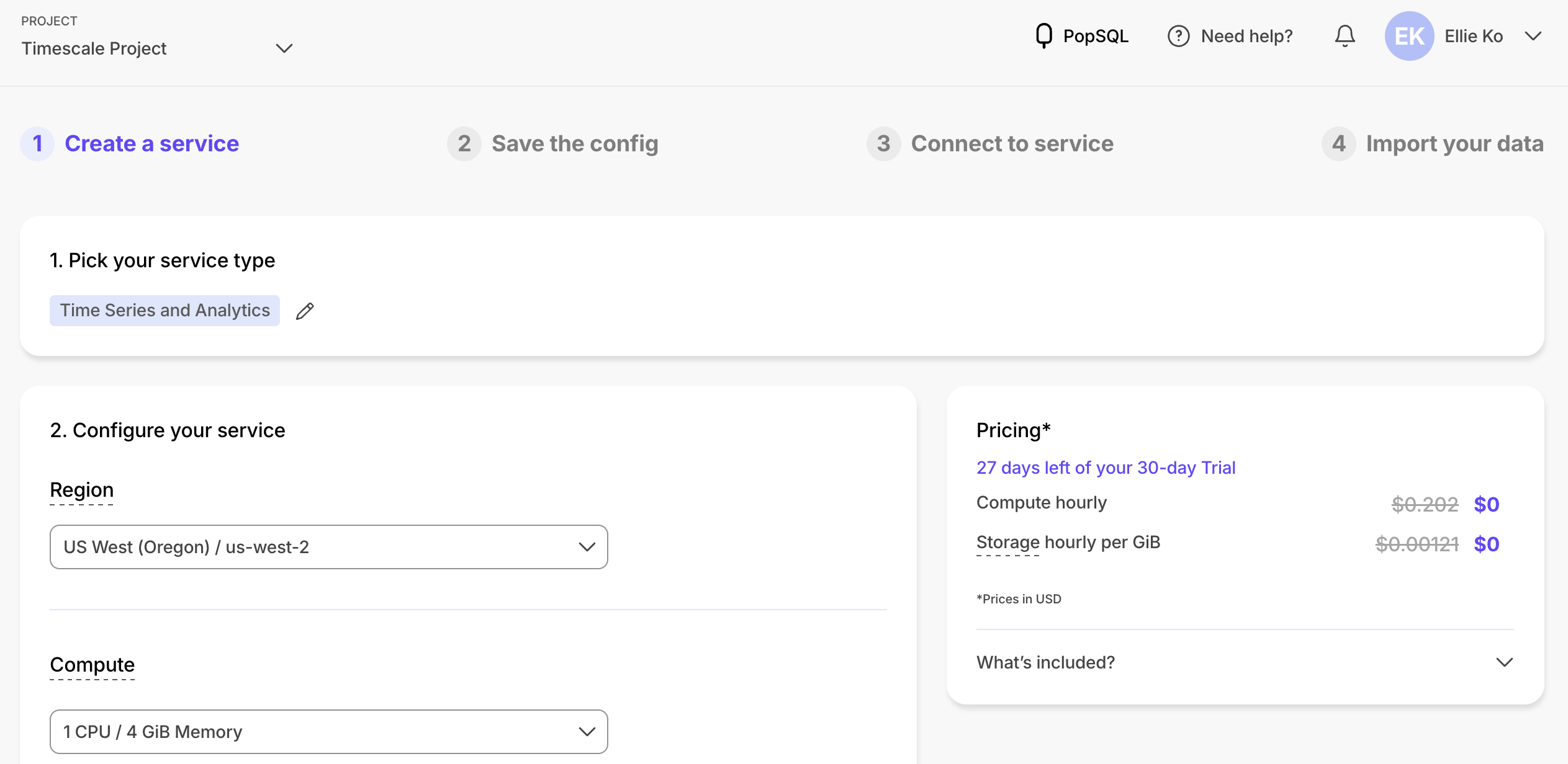
To start with Timescale DB, sign up here, and click New service in your dashboard.
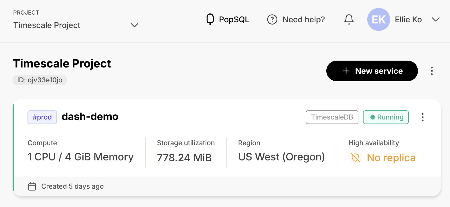
Configure your service:
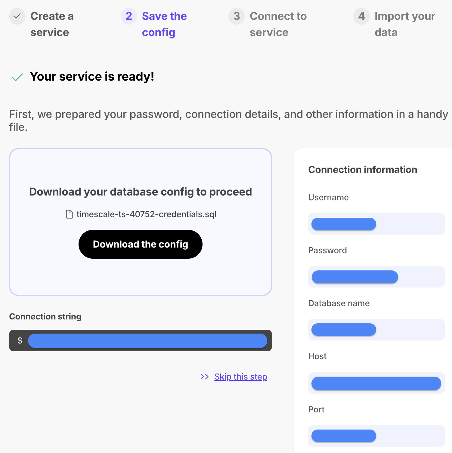
Now save your connection information. This is crucial as you will need this information to connect both your backend and frontend scripts to the database.
Binance offers both REST API and WebSocket APIs. For this project, the WebSocket method is more optimal because of its faster data updates. Specifically, we will use the Aggregate Trade Stream, which delivers market trade information aggregated by price and side every 100 milliseconds. For more details about the Aggregate Trade Stream, visit the official documentation.
Below is an example of the response from the WebSocket request to wss://data-stream.binance.vision/ws/btcusdt@aggTrade. In our application, we will utilize the Price (‘p’) and Trade time (‘T’) from this data.
{
  "e": "aggTrade",        // Event type
  "E": 1723588247081,     // Event time
  "s": "BTCUSDT",         // Symbol
  "a": 3114876932,        // Aggregate trade ID
  "p": "60610.00000000",  // Price
  "q": "0.00094000",      // Quantity
  "f": 3743607521,        // First trade ID
  "l": 3743607521,        // Last trade ID
  "T": 1723588247080,     // Trade time
  "m": True,              // Is the buyer the market maker?
}
Now that we have all the necessary components, including DB connection details and the WebSocket API endpoint, let’s dive into the implementation of websocket_backend.py.
Start by importing the necessary libraries. If any are missing, install them using pip install <library>.
import asyncio, asyncpg, datetime, json, os
from websockets import connect
from dotenv import load_dotenv  # if you want to use .env for loading environment variables
You can either manually set your DB connection details as environment variables using export DB_USER=<USERNAME>, or utilize a .env file in your working directory and load it via load_dotenv(".env") at the beginning of websocket_backend.py. Your .env file should be formatted as follows:
DB_USER=<USERNAME>
DB_PASSWORD=<PASSWORD>
DB_NAME=<DATABASE_NAME>
DB_HOST=<HOST>
DB_PORT=<PORT>
Define the setup_db function to create a table for time and price data. For TimescaleDB, convert this table into a hypertable to efficiently manage time-series data. A hypertable is an abstraction in TimescaleDB that automatically partitions data into smaller chunks based on time intervals. This partitioning optimizes query speeds and simplifies the scaling process, making it ideal for managing continuously growing time-series data.
Note: For databases that do not support hypertables, enhance query performance by creating an index on trades(time). This index optimizes data retrieval based on time, improving the efficiency of time-based queries.
async def setup_db():
    db_user = os.getenv('DB_USER')
    db_password = os.getenv('DB_PASSWORD')
    db_host = os.getenv('DB_HOST')
    db_port = os.getenv('DB_PORT')
    db_name = os.getenv('DB_NAME')

    if not all([db_user, db_password, db_host, db_port, db_name]):
        raise ValueError("Database connection details are not fully set in environment variables")

    conn = await asyncpg.connect(user=db_user,
                                password=db_password,
                                database=db_name,
                                host=db_host,
                                port=db_port)
    await conn.execute("DROP TABLE IF EXISTS trades")
    await conn.execute("""
        CREATE TABLE trades(
            time TIMESTAMP NOT NULL,
            price DOUBLE PRECISION
        )
    """)
    await conn.execute("SELECT create_hypertable('trades', 'time')")
    await conn.close()
Define insert_data to capture and store data from the API in batches of 5.
async def insert_data(url, db_conn):
    trades_buffer = []
    async with connect(url) as websocket:
        while True:
            data = await websocket.recv()
            data = json.loads(data)
            trades_buffer.append((datetime.datetime.fromtimestamp(data['T']/1000.0), float(data['p'])))
            print(trades_buffer[-1])
            # Write in batches of 5
            if len(trades_buffer) > 5:
                await db_conn.executemany("""INSERT INTO trades(time, price) VALUES ($1, $2)""", trades_buffer)
                trades_buffer = []
Finally, execute the setup and data insertion functions with the correct parameters.
async def main():
    url_binance = "wss://data-stream.binance.vision/ws/btcusdt@aggTrade"
    await setup_db()
    db_conn = await asyncpg.connect(user=os.getenv("DB_USER"),
                                    password=os.getenv("DB_PASSWORD"),
                                    database=os.getenv("DB_NAME"),
                                    host=os.getenv("DB_HOST"),
                                    port=os.getenv("DB_PORT"))
    try:
        await insert_data(url_binance, db_conn)
    finally:
        await db_conn.close()

if __name__ == "__main__":
    asyncio.run(main())
Run this complete script locally via python websocket_backend.py to see if it successfully prints out the real-time data.
Additionally, you can check how the data looks in the TimeScale DB console with the following query:
tsdb=> SELECT * FROM trades LIMIT 5;
          time           |  price
-------------------------+----------
 2024-08-15 23:43:31.181 | 58432.51
 2024-08-15 23:43:31.244 |  58432.5
 2024-08-15 23:43:31.345 |  58432.5
 2024-08-15 23:43:31.345 |  58432.5
 2024-08-15 23:43:31.345 |  58432.5
(5 rows)
Finally! It’s time to explore our Dash app.
Create a new file named app.py and start by importing the necessary libraries. If any libraries are missing, you can install them via pip install <library>.
from dash import html, dcc, Output, Input, Dash
import dash_bootstrap_components as dbc
import os, psycopg2
Define a lambda function to initialize graph layouts, opting for a dark theme.
graph_title1 = "Price Change: 5-Minute Rolling Window (BTC/USDT)"
graph_title2 = "Aggregate Trades per Minute: 5-Minute Rolling Window"

default_fig = lambda title: dict(
    data=[{'x': [], 'y': [], 'name': title}],
    layout=dict(
        title=dict(text=title, font=dict(color='white')),
        xaxis=dict(autorange=True, tickformat="%H:%M:%S", color='white', nticks=8),
        yaxis=dict(autorange=True, color="white"),
        paper_bgcolor="#2D2D2D",
        plot_bgcolor="#2D2D2D"
    ))
Initialize the Dash application using the CYBORG theme from dash_bootstrap_components to have a black theme. If you’re interested in different themes for your Dash application, explore options here.
The app layout will include (1) H1 for the app title, (2) H2 to display the current Bitcoin price, (3) two graphs with distinct IDs and styles for visualizing data updates, and lastly, (4) the key component in our app: dcc.Interval.
dcc.Interval is what enables us to fire a callback periodically. Set its interval property to 4000 milliseconds. This setup updates our graphs every 4 seconds.
app = Dash(external_stylesheets=[dbc.themes.CYBORG])
server = app.server
app.layout = html.Div([
    html.H1("Live Bitcoin Monitoring App",
            style={"text-align":"center", "padding-top":"20px", "padding-bottom":"20px"}),
    html.Hr(),
    html.H2(id="price-ticker",
            style={"text-align":"center", "padding-top":"10px", "padding-bottom":"10px"}),
    dcc.Graph(id="graph-price-change", figure=default_fig(graph_title1)),
    dcc.Graph(id="graph-agg-per-min", figure=default_fig(graph_title2)),
    dcc.Interval(id="update", interval=4000),
    ])
Define a function to fetch data from the PostgreSQL database. Ensure that environment variables for DB connection details are set.
# Cache the previous time to avoid fetching the same data multiple times
previous_time = None

# Function to fetch data from the database
def fetch_data():
    global previous_time
    # Construct the connection string
    db_user = os.getenv('DB_USER')
    db_password = os.getenv('DB_PASSWORD')
    db_host = os.getenv('DB_HOST')
    db_port = os.getenv('DB_PORT')
    db_name = os.getenv('DB_NAME')

    if not all([db_user, db_password, db_host, db_port, db_name]):
        return None, "Database connection details are not fully set in environment variables"

    connection_string = f"postgresql://{db_user}:{db_password}@{db_host}:{db_port}/{db_name}"
    try:
        with psycopg2.connect(connection_string) as conn:
            cursor = conn.cursor()
            cursor.execute("""
                SELECT *
                FROM trades
                WHERE time >= (
                    SELECT MAX(time)
                    FROM trades
                ) - INTERVAL '1 minute';
            """)
            rows = cursor.fetchall()

            # Check if there was no new data available
            if not rows or (previous_time and rows[0][0] <= previous_time):
                print("No data available - Are you running websocket_backend.py?")
                return None, "No data available"

            previous_time = rows[0][0]

            return rows, None

    except psycopg2.Error as e:
        print(f"Database connection error: {e}")
        return None, "Database connection error"
Set up a callback to extend the data in our graphs and update the price ticker based on fetched data, updating every 4 seconds as defined by our dcc.Interval.
If the intention was to redraw the entire plot, you would use the figure property of the dcc.Graph component in the callback function. However, since our goal is to append a new data point to the existing graph, we utilize the extendData property. For more information about the properties of dcc.Graph that you can leverage, check out this documentation.
# Callback to extend the data in the graphs
@app.callback(
        Output("graph-price-change", "extendData"),
        Output("graph-agg-per-min", "extendData"),
        Output("price-ticker", "children"),
        Input("update", "n_intervals"),
        )
def update_data(intervals):
    rows, msg = fetch_data()
    if rows == None:
        return None, None, msg

    current_price = rows[0][1]
    total_trades = len(rows)
    new_data_price_change = dict(x=[[rows[0][0]]], y=[[current_price]])
    new_data_agg_per_min = dict(x=[[rows[0][0]]], y=[[total_trades]])

    # (new data, trace to add data to, number of elements to keep)
    return ((new_data_price_change, [0], 75),
            (new_data_agg_per_min, [0], 75),
            f"Current BTC price: {current_price}")
Finally, run the server to make our application live:
if __name__ == "__main__":
    app.run_server(debug=True)
Now you are done with app.py! Run python app.py to launch your Dash app at http://127.0.0.1:8050/. If your websoket_backend.py is successfully running, you should see new data points appended to your Dash app every 4 seconds or at the interval you’ve set.
Deploying your Dash application on Ploomber Cloud is straightforward and ensures your app can be accessed by users anytime, anywhere. Ploomber Cloud not only provides deployment solutions but also robust security features, including password protection and application secrets. If you haven’t created an account yet, start for free here and deploy your app today!
Ploomber Cloud supports two deployment methods:
To deploy your Dash app on Ploomber Cloud, you need:
app.pyrequirements.txt.env (only for CLI method)The above requirements.txt includes all libraries you need for both backend and Dash app. To deploy your Dash app, delete libraries from requirements.txt that are not needed. Your requirements.txt should be:
dash
dash-bootstrap-components
psycopg2-binary
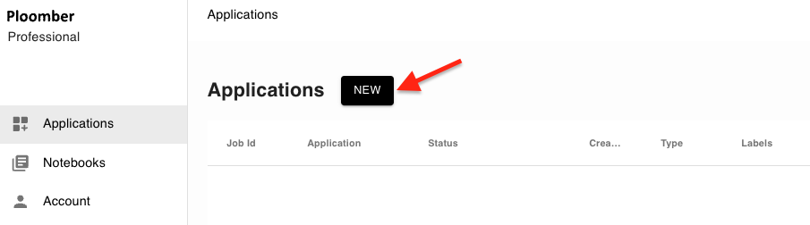
Log into your Ploomber Cloud account.
Click the NEW button:
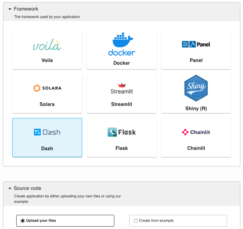
Select the Dash option, and upload your code (app.py and requirements.txt) as a zip file in the source code section:
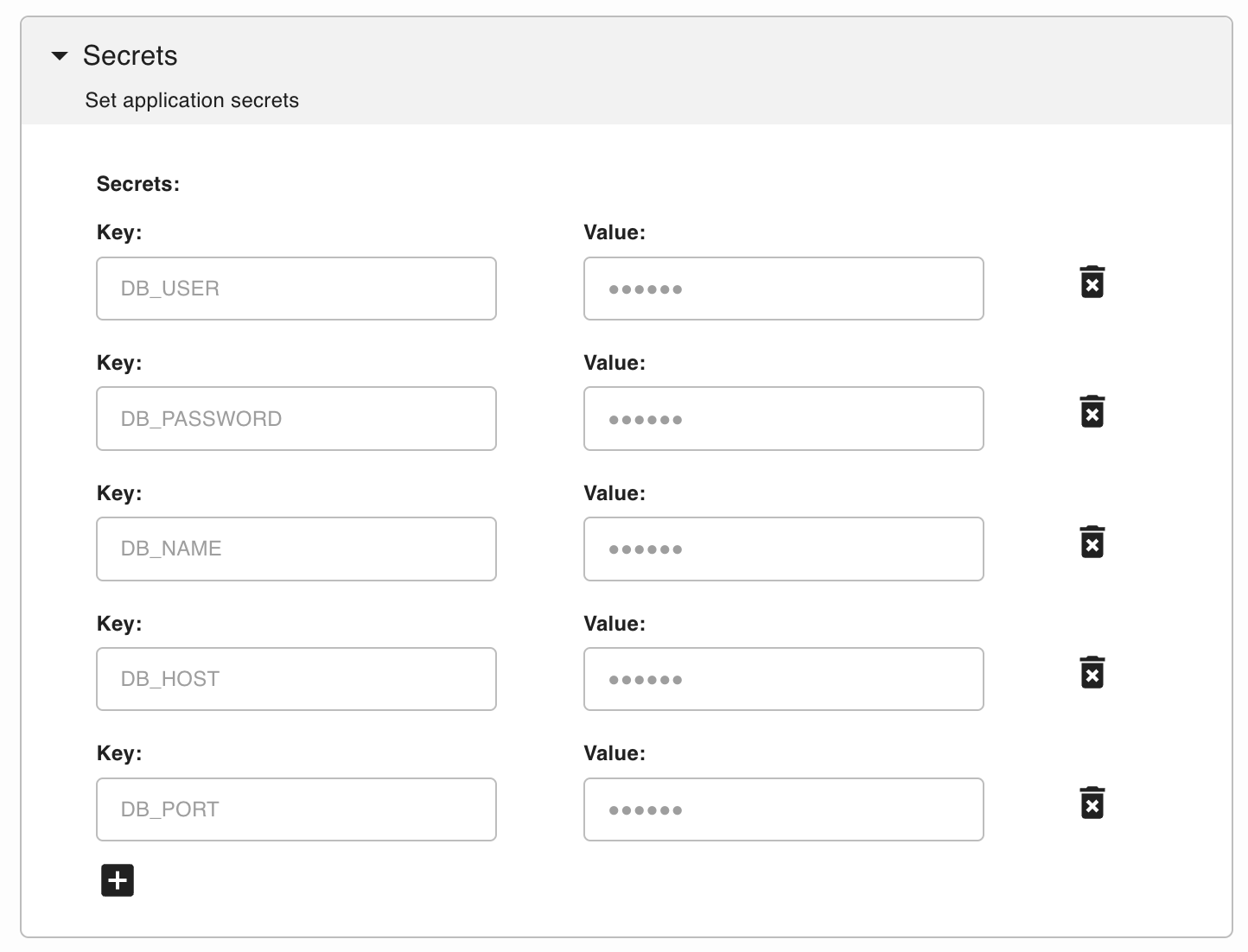
In the secret section, add your database’s connection details as environment variables required for our app.
After optionally customizing some settings, click CREATE.
If you haven’t installed ploomber-cloud, run:
pip install ploomber-cloud
Set your API key following this documentation.
ploomber-cloud key YOURKEY
Navigate to your project directory where your files are located:
cd <project-name>
Or, if you prefer downloading the explained code and make changes there, run the following command:
ploomber-cloud examples dash/dash-live-updates
Note: Make sure you only separate files for your Dash app deployment. Specifically, you need app.py, an updated requirements.txt, and a .env file for your database connection.
Then, initialize the project and confirm the inferred project type (Dash) when prompted:
(testing_dash_app) ➜ ploomber-cloud init                    ✭ ✱
Initializing new project...
Inferred project type: 'dash'
Is this correct? [y/N]: y
Your app '<id>' has been configured successfully!
To configure resources for this project, run 'ploomber-cloud resources' or to deploy with default configurations, run 'ploomber-cloud deploy'
Deploy your application and monitor the deployment at the provided URL:
(testing_dash_app) ➜  cloud ploomber-cloud deploy                  ✭ ✱
Compressing app...
Reading .env file...
Adding the following secrets to the app: DB_USER, DB_PASSWORD, DB_NAME, DB_HOST, DB_PORT,
Adding app.py...
Ignoring file: ploomber-cloud.json
Adding requirements.txt...
App compressed successfully!
Deploying project with id: <id>...
The deployment process started! Track its status at: https://www.platform.ploomber.io/applications/<id>/<job_id>
For more details, see this documentation.
Let’s take a look at your deployed app. The GIF below is sped up three times faster than real-time to demonstrate functionality more quickly; however, in actual use, your app will add a new data point every 4 seconds.
In this tutorial, we demonstrated how to efficiently update Dash graphs with real-time data and deployed our Bitcoin Monitoring App on Ploomber Cloud for global access. This approach ensures smooth updates without the need to redraw graphs completely, enhancing performance and user experience.
Explore further with Dash and Ploomber Cloud to build and deploy dynamic applications effortlessly. For additional resources and guides, check out our website!
Seamless deployment for data scientists and developers. Ploomber handles infrastructure so you focus on building. Secure and scalable—from personal projects to enterprise apps. Support for Streamlit, Dash, Docker, and AI-powered applications. Because life's too short for deployment headaches.