


Struggling to get Python packages installed? Get a pre-configured JupyterLab instance for free! Sign up for Ploomber Platform!
Clustering techniques allow us to identify subgroups (or clusters) in data such that data points in each same cluster are very similar to each other, and other data points in separate clusters have different characteristics. Clustering techniques can be used in various fields of study and real-life applications, such as data mining, bioinformatics, image processing, recommendation engines, and more.
In this post, we will create a clustering model that will be trained with 20 different parameters, ending up with 20 different models. Then, we will plot the elbow curve using the results of the trained models. As an important addition, we are going to use Ploomber Cloud to train these 20 models, making the best use of cloud capabilities for free.
To evaluate the 20 models once trained, we will use the elbow method, as it will allow us to identify the optimal number of clusters in our data. The elbow method is a widely used heuristic method in cluster analysis. It is used, as expected, to determine the number of clusters in a dataset.
The method consists of plotting the explained variation as a function of the number of clusters and selecting the elbow of the curve as the number of clusters to use. This method is very useful, as you can even use this same approach in other data-driven models. You can read more details here and here.
We have prepared a functional notebook for you. This notebook contains code to run 20 models in the cloud, now that we recently introduced Ploomber Cloud Notebooks.
You can download the prepared notebook by opening a terminal and running the following command:
curl https://raw.githubusercontent.com/ploomber/posts/master/elbow-curve/cluster.ipynb -o cluster.ipynb
Now that you have downloaded the notebook, let’s explore the code in it.
Note: If you want to explore/modify the contents of the notebook, you can do so by opening the notebook with Jupyter (by running
jupyter labin your terminal, please note that Jupyter Lab needs to be installed).
The code in the notebook contains a set of instructions to import functions to create synthetic data and run a clustering algorithm known as K-Means. The main part is shown as follows, and as we can see, it is run with a specified number of clusters, and then we measure the performance over the generated data by using the sum of squares:
model = KMeans(n_clusters=n_clusters, random_state=0)

sum_of_squares = abs(model.fit(X).score(X))
What is important to us, is that the notebook will run this algorithm for a specified number of clusters, let’s say, for clusters from 1 to 20. As you can see, the notebook only seems to run the previous code to create and fit the model once, and here’s where Ploomber Cloud’s magic comes to play.
To run this model for 20 different clusters, we need to specify the output prefix and the number of clusters that will be taken as variables (in a grid execution). This must be specified in the first cell of the notebook, as we did in the notebook we prepared for you.
If you open the notebook, you will find the following in the first cell:
prefix: elbow-curve

grid:
  n_clusters: [1, 2, 3, 4, 5, 6, 7, 8, 9, 10, 11, 12, 13, 14, 15, 16, 17, 18, 19, 20]
As mentioned, this code will take the prefix name to generate the results for each model (elbow-curve-0, …, elbow-curve-19), by using the values specified in the grid in the n_clusters list.
Next to this setup, the name of the parameter that is passed to the K-Means algorithm needs to be set. We do this by adding another cell with the following:
# PARAMETERS
n_clusters = 1
This is the variable that takes the different values from the grid and is passed to
model = KMeans(n_clusters=n_clusters, random_state=0)
as a parameter of the model.
This is all we need to execute this model 20 times, in parallel, with a different number of clusters each time by running the notebook in the cloud, so let’s run it in Ploomber Cloud! 🔥
If you want to dive more into the notebook structure, we highly recommend you to read our documentation on Running experiments in parallel.
Now that we downloaded and explored the notebook, we can proceed to upload it to Ploomber Cloud. For this, we will need to have the latest version of Ploomber installed and you also need to set up your API Key.
You can install the latest version by running the following in your terminal:
pip install --upgrade ploomber
Once you have the latest version of Ploomber installed and your API Key configured, we can proceed to run the notebook in the cloud. Run the following in your terminal:
ploomber cloud nb cluster.ipynb
Console output (1/1):
Uploading cluster-14abd526.ipynb...
Triggering execution of cluster-14abd526.ipynb...
Done. Monitor Docker build process with:
  $ ploomber cloud logs 94d683bd-1a4a-4a70-98aa-f4cb53efc67c --image --watch
This will upload and run the notebook in Ploomber Cloud using your account.
After a minute, the 20 models should finish fitting:
ploomber cloud status @latest
Console output (1/1):
taskid                      name            runid                       status
--------------------------  --------------  --------------------------  --------
b9925ac5-2140-4e63-a611-30  elbow-curve-10  94d683bd-1a4a-4a70-98aa-f4  finished
b0014ba61f                                  cb53efc67c
99017f30-d656-4647-81e2-4f  elbow-curve-14  94d683bd-1a4a-4a70-98aa-f4  finished
ab39dae0ea                                  cb53efc67c
958eb37e-a632-4332-a97d-f8  elbow-curve-5   94d683bd-1a4a-4a70-98aa-f4  finished
3a92f5b1d3                                  cb53efc67c
66953fc0-2536-41b0-ad57-93  elbow-curve-1   94d683bd-1a4a-4a70-98aa-f4  finished
1471d76901                                  cb53efc67c
386caa75-b015-40f9-86ac-5c  elbow-curve-6   94d683bd-1a4a-4a70-98aa-f4  finished
c0e5b5dd9e                                  cb53efc67c
cdb641c2-1bf3-46c9-81db-    elbow-curve-2   94d683bd-1a4a-4a70-98aa-f4  finished
aad34fb6a090                                cb53efc67c
eccab590-5ed7-4e21-8127-81  elbow-curve-12  94d683bd-1a4a-4a70-98aa-f4  finished
b14812fa99                                  cb53efc67c
eb3b69ec-c408-4f0b-ac2b-a0  elbow-curve-3   94d683bd-1a4a-4a70-98aa-f4  finished
b36fb9c94b                                  cb53efc67c
3b9ac45d-3540-4d55-9e59-9e  elbow-curve-13  94d683bd-1a4a-4a70-98aa-f4  finished
7540a3fb9d                                  cb53efc67c
de97fbf8-5155-4900-aec7-41  elbow-curve-18  94d683bd-1a4a-4a70-98aa-f4  finished
84bcafde02                                  cb53efc67c
d6b187ff-0c3b-4e29-a323-f1  elbow-curve-9   94d683bd-1a4a-4a70-98aa-f4  finished
99359a64f9                                  cb53efc67c
317e8b27-ccdc-49a6-b6e1-c2  elbow-curve-7   94d683bd-1a4a-4a70-98aa-f4  finished
24bf6688f5                                  cb53efc67c
3b9c43a0-bafa-4c3f-a461-2c  elbow-curve-16  94d683bd-1a4a-4a70-98aa-f4  finished
e3f65dc1ba                                  cb53efc67c
72e6e49a-4020-45b0-bc0d-0c  elbow-curve-0   94d683bd-1a4a-4a70-98aa-f4  finished
a8a2fd7b95                                  cb53efc67c
b4b1085f-4d67-4b81-9dcd-    elbow-curve-19  94d683bd-1a4a-4a70-98aa-f4  finished
bcb1b57f2f89                                cb53efc67c
897ba1e7-b471-483a-a34c-e5  elbow-curve-4   94d683bd-1a4a-4a70-98aa-f4  finished
c4bb035b01                                  cb53efc67c
6537448b-ed1d-4f7b-8756-79  elbow-curve-8   94d683bd-1a4a-4a70-98aa-f4  finished
46b2349d4e                                  cb53efc67c
09c971aa-85ba-44c2-b972-22  elbow-curve-17  94d683bd-1a4a-4a70-98aa-f4  finished
92f901d528                                  cb53efc67c
6ee06d3e-841c-4973-833a-f5  elbow-curve-11  94d683bd-1a4a-4a70-98aa-f4  finished
dabab45141                                  cb53efc67c
f66ec42a-069a-420b-8e69-20  elbow-curve-15  94d683bd-1a4a-4a70-98aa-f4  finished
580af42983                                  cb53efc67c

Pipeline finished. Check outputs:
  $ ploomber cloud products
Once the models have finished running in the cloud, the results are stored in your instance and they can be easily downloaded with the following command:
ploomber cloud download 'elbow-curve/*'
Console output (1/1):
Writing file into path elbow-curve/output/notebook-n_clusters=19-18.ipynb
Writing file into path elbow-curve/output/notebook-n_clusters=4-3.ipynb
Writing file into path elbow-curve/output/notebook-n_clusters=10-9.ipynb
Writing file into path elbow-curve/output/notebook-n_clusters=17-16.ipynb
Writing file into path elbow-curve/output/notebook-n_clusters=3-2.ipynb
Writing file into path elbow-curve/output/notebook-n_clusters=14-13.ipynb
Writing file into path elbow-curve/output/notebook-n_clusters=16-15.ipynb
Writing file into path elbow-curve/output/notebook-n_clusters=18-17.ipynb
Writing file into path elbow-curve/output/notebook-n_clusters=1-0.ipynb
Writing file into path elbow-curve/output/notebook-n_clusters=7-6.ipynb
Writing file into path elbow-curve/output/.notebook-n_clusters=10-9.ipynb.metadata
Writing file into path elbow-curve/output/notebook-n_clusters=15-14.ipynb
Writing file into path elbow-curve/output/notebook-n_clusters=2-1.ipynb
Writing file into path elbow-curve/output/.notebook-n_clusters=1-0.ipynb.metadata
Writing file into path elbow-curve/output/notebook-n_clusters=8-7.ipynb
Writing file into path elbow-curve/output/.notebook-n_clusters=12-11.ipynb.metadata
Writing file into path elbow-curve/output/.notebook-n_clusters=15-14.ipynb.metadata
Writing file into path elbow-curve/output/notebook-n_clusters=6-5.ipynb
Writing file into path elbow-curve/output/notebook-n_clusters=5-4.ipynb
Writing file into path elbow-curve/output/notebook-n_clusters=12-11.ipynb
Writing file into path elbow-curve/output/.notebook-n_clusters=18-17.ipynb.metadata
Writing file into path elbow-curve/output/.notebook-n_clusters=17-16.ipynb.metadata
Writing file into path elbow-curve/output/.notebook-n_clusters=14-13.ipynb.metadata
Writing file into path elbow-curve/output/notebook-n_clusters=11-10.ipynb
Writing file into path elbow-curve/output/notebook-n_clusters=13-12.ipynb
Writing file into path elbow-curve/output/notebook-n_clusters=20-19.ipynbWriting file into path elbow-curve/output/.notebook-n_clusters=16-15.ipynb.metadata

Writing file into path elbow-curve/output/.notebook-n_clusters=20-19.ipynb.metadataWriting file into path elbow-curve/output/.notebook-n_clusters=13-12.ipynb.metadata

Writing file into path elbow-curve/output/.notebook-n_clusters=3-2.ipynb.metadata
Writing file into path elbow-curve/output/.notebook-n_clusters=19-18.ipynb.metadata
Writing file into path elbow-curve/output/.notebook-n_clusters=2-1.ipynb.metadata
Writing file into path elbow-curve/output/.notebook-n_clusters=4-3.ipynb.metadata
Writing file into path elbow-curve/output/notebook-n_clusters=9-8.ipynb
Writing file into path elbow-curve/output/.notebook-n_clusters=9-8.ipynb.metadata
Writing file into path elbow-curve/output/.notebook-n_clusters=8-7.ipynb.metadata
Writing file into path elbow-curve/output/.notebook-n_clusters=6-5.ipynb.metadataWriting file into path elbow-curve/output/.notebook-n_clusters=5-4.ipynb.metadata

Writing file into path elbow-curve/output/.notebook-n_clusters=7-6.ipynb.metadata
Writing file into path elbow-curve/output/.notebook-n_clusters=11-10.ipynb.metadata
You will find all the downloaded contents inside the elbow-curve/ folder on your local machine.
Now, we will create an elbow curve to explore the results of the models and we will then decide the optimal number of clusters. For this, we will use sklearn-evaluation, as this package includes many tools for machine learning model evaluation, such as tables, plots, HTML reports, and more.
Specifically, we will use the notebook collection feature, as it allows us to retrieve results from previously executed notebooks to compare them. We only need to tag cells whose output we want to extract and use for the comparison, each tag then becomes a key in the notebook collection. For more details on adding tags, you can see this.
Let’s now proceed to import the needed packages:
from glob import glob

import numpy as np
from sklearn_evaluation import NotebookCollection
from sklearn_evaluation import plot
Let’s create a NotebookCollection from the notebooks we executed in the cloud (now downloaded and stored locally):
nbs = NotebookCollection(paths=glob('elbow-curve/**/*.ipynb'))
We proceed to grab the outputs from the cells we tagged:
n_clusters = list(nbs['n-clusters'].values())
elapsed = list(nbs['elapsed'].values())
sum_of_squares = list(nbs['sum-of-squares'].values())
And finally, we plot the elbow curve with plot.elbow_curve_from_results:
_ = plot.elbow_curve_from_results(n_clusters, sum_of_squares, elapsed)
Console output (1/1):
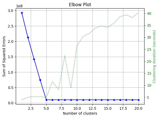
Please note that we used the function
plot.elbow_curve_from_resultsas we ran the prepared notebook in Ploomber Cloud, but you can run multiple models locally and use the elbow method withplot.elbow_curve(see here for more info).
From the plot, we can note that the optimal number of clusters is 5.
Congratulations! 🎉
So far, you were able to train a model with 20 different parameters, ending with 20 different models to compare. As you can see, Ploomber Cloud is very useful to parametrize notebook runs. Finally, once you trained and downloaded the results from Ploomber Cloud, you were able to compare the results by plotting the elbow curve for the 20 different models.
If you want to know more about Ploomber Cloud, you can check out our docs and join our awesome community to ask any questions.
Seamless deployment for data scientists and developers. Ploomber handles infrastructure so you focus on building. Secure and scalable—from personal projects to enterprise apps. Support for Streamlit, Dash, Docker, and AI-powered applications. Because life's too short for deployment headaches.