


I spent about six years working as a data scientist and tried to use MLflow several times (and others as well) to track my experiments; however, every time I tried using it, I abandoned it a few days after.
There were a few things I didn’t like: it seemed too much to have to start a web server to look at my experiments, and I found the query feature extremely limiting (if my experiments are stored in a SQL table, why not allow me to query them with SQL).
I also found comparing the experiments limited. I rarely have a project where a single (or a couple of) metric(s) is enough to evaluate a model. It’s mostly a combination of metrics and evaluation plots that I need to look at to assess a model. Furthermore, the numbers/plots themselves have no value in isolation; I need to benchmark them against a base model, and doing model comparisons at this level was pretty slow from the GUI.
So I decided to develop an experiment tracker that would satisfy those needs: no need to run a server, SQL as the query language, flexible comparison capabilities, and no need to add custom code. This version is the first release! So please take it for a spin and share your feedback with us on GitHub or Slack; we want to build the most powerful and flexible experiment tracker!
First, let’s install the required packages:
pip install ploomber-engine sklearn-evaluation jupytext --upgrade
Now, let’s download the sample script we’ll use:
curl -O https://raw.githubusercontent.com/ploomber/posts/master/experiment-tracking/fit.py
Console output (1/1):
% Total    % Received % Xferd  Average Speed   Time    Time     Time  Current
                                 Dload  Upload   Total   Spent    Left  Speed
100  1718  100  1718    0     0   4954      0 --:--:-- --:--:-- --:--:--  4965
For this example, we’ll train several random forest models using scikit-learn and then use the experiment tracker to evaluate results. However, remember that the tool is generic enough to be used in other data domains like bioinformatics or analytics.
Let’s create our grid of parameters:
from ploomber_engine.tracking import track_execution
from sklearn.model_selection import ParameterGrid

grid = ParameterGrid(
    dict(
        n_estimators=[5, 10, 15, 25, 50, 100],
        model_type=["sklearn.ensemble.RandomForestClassifier"],
        max_depth=[5, 10, None],
        criterion=["gini", "entropy", "log_loss"],
    )
)
Let’s now execute the script multiple times, one per set of parameters, and store the results in the experiments.db SQLite database:
for idx, p in enumerate(grid):
    if (idx + 1) % 10 == 0:
        print(f"Executed {idx + 1}/{len(grid)} so far...")

    track_execution("fit.py", parameters=p, quiet=True, database="experiments.db")
Console output (1/1):
Executed 10/54 so far...
Executed 20/54 so far...
Executed 30/54 so far...
Executed 40/54 so far...
Executed 50/54 so far...
Note: we’re running a Python script, but Jupyter notebooks (.ipynb) are also supported.
If you prefer so, you can also execute scripts from the terminal:
python -m ploomber_engine.tracking fit.py \
    -p n_estimators=100,model_type=sklearn.ensemble.RandomForestClassifier,max_depth=10
If you look at the script’s source code, you’ll see that there are no extra imports or calls to log the experiments, it’s a vanilla Python script.
The tracker runs the code, and it logs everything that meets any of the following conditions:
accuracy = accuracy_score(y_test, y_pred)
accuracy
plot.confusion_matrix(y_test, y_pred)
Note that logs happen in groups (not line-by-line). A group is defined as a contiguous set of lines delimited with line breaks:
# first group
accuracy = accuracy_score(y_test, y_pred)
accuracy

# second group
plot.confusion_matrix(y_test, y_pred)
Regular Python objects are supported (numbers, strings, lists, dictionaries), and any object with a rich representation will also work (e.g., matplotlib charts).
After finishing executing the experiments, we can initialize our database (experiments.db) and explore the results:
from sklearn_evaluation import SQLiteTracker

tracker = SQLiteTracker("experiments.db")
Since this is a SQLite database, we can use SQL to query our data using the .query method. By default, we get a pandas.DataFrame:
df = tracker.query(
    """
SELECT *
FROM experiments
LIMIT 5
"""
)

type(df)
Console output (1/1):
pandas.core.frame.DataFrame
df.head(3)
Console output (1/1):
| created | parameters | comment | |
|---|---|---|---|
| uuid | |||
| 15b173ac | 2022-11-15 20:09:15 | {"criterion": "gini", "max_depth": 5, "model_t... | None |
| f30a65f0 | 2022-11-15 20:09:17 | {"criterion": "gini", "max_depth": 5, "model_t... | None |
| 85684951 | 2022-11-15 20:09:18 | {"criterion": "gini", "max_depth": 5, "model_t... | None |
The logged parameters are stored in the parameters column. This column is a JSON object, and we can inspect the JSON keys with the .get_parameters_keys() method:
tracker.get_parameters_keys()
Console output (1/1):
['accuracy',
 'classification_report',
 'confusion_matrix',
 'criterion',
 'f1',
 'max_depth',
 'model_type',
 'n_estimators',
 'precision',
 'precision_recall',
 'recall']
To get a sample query, we can use the .get_sample_query() method:
print(tracker.get_sample_query())
Console output (1/1):
SELECT
    uuid,
    json_extract(parameters, '$.accuracy') as accuracy,
    json_extract(parameters, '$.classification_report') as classification_report,
    json_extract(parameters, '$.confusion_matrix') as confusion_matrix,
    json_extract(parameters, '$.criterion') as criterion,
    json_extract(parameters, '$.f1') as f1,
    json_extract(parameters, '$.max_depth') as max_depth,
    json_extract(parameters, '$.model_type') as model_type,
    json_extract(parameters, '$.n_estimators') as n_estimators,
    json_extract(parameters, '$.precision') as precision,
    json_extract(parameters, '$.precision_recall') as precision_recall,
    json_extract(parameters, '$.recall') as recall
    FROM experiments
LIMIT 10
Let’s perform a simple query that extracts our metrics, sorts by F1 score, and returns the top three experiments:
tracker.query(
    """
SELECT
    uuid,
    json_extract(parameters, '$.f1') as f1,
    json_extract(parameters, '$.accuracy') as accuracy,
    json_extract(parameters, '$.criterion') as criterion,
    json_extract(parameters, '$.n_estimators') as n_estimators,
    json_extract(parameters, '$.precision') as precision,
    json_extract(parameters, '$.recall') as recall
FROM experiments
ORDER BY f1 DESC
LIMIT 3
""",
    as_frame=False,
    render_plots=False,
)
Console output (1/1):
| uuid | f1 | accuracy | criterion | n_estimators | precision | recall |
|---|---|---|---|---|---|---|
| efa894dd | 0.806188 | 0.798788 | gini | 100 | 0.774103 | 0.841048 |
| ad8fb523 | 0.804184 | 0.795758 | entropy | 100 | 0.768889 | 0.842875 |
| 93154ceb | 0.800583 | 0.792727 | log_loss | 100 | 0.767897 | 0.836175 |
Plots are essential for evaluating our analysis, and the experiment tracker can log them automatically. So let’s pull the top 2 experiments (by F1 score) and get their confusion matrices, precision-recall curves, and classification reports. Note that we passed as_frame=False and render_plots=True to the .query method:
top_two = tracker.query(
    """
SELECT
    uuid,
    json_extract(parameters, '$.f1') as f1,
    json_extract(parameters, '$.confusion_matrix') as confusion_matrix,
    json_extract(parameters, '$.precision_recall') as precision_recall,
    json_extract(parameters, '$.classification_report') as classification_report
FROM experiments
ORDER BY f1 DESC
LIMIT 2
""",
    as_frame=False,
    render_plots=True,
)

top_two
Console output (1/1):
| uuid | f1 | confusion_matrix | precision_recall | classification_report |
|---|---|---|---|---|
| efa894dd | 0.806188 |  |  |  |
| ad8fb523 | 0.804184 |  |  |  |
If you want to zoom into a couple of experiment plots, you can select one and create a tab view. First, let’s retrieve the confusion matrices from the top 2 experiments:
top_two.get("confusion_matrix")
Console output (1/1):
The buttons in the top bar allow us to switch between the two plots of the selected experiments. We can do the same with the precision-recall curve:
top_two.get("precision_recall")
Console output (1/1):
Note that the tabs will take the value of the first column in our query (in our case, the experiment ID). So let’s switch them to show the F1 score via the index_by argument:
top_two.get("classification_report", index_by="f1")
Console output (1/1):
Using SQL gives us power and flexibility to answer sophisticated questions about our experiments.
For example, let’s say we want to know the effect of the number of trees (n_estimators) on our metrics. We can quickly write a SQL that aggregates by n_estimators and computes the mean of all our metrics; then, we can plot the values.
First, let’s run the query. Note that we’re passing as_frame=True so we get a pandas.DataFrame we can manipulate:
df = tracker.query(
    """
SELECT
    json_extract(parameters, '$.n_estimators') as n_estimators,
    AVG(json_extract(parameters, '$.accuracy')) as accuracy,
    AVG(json_extract(parameters, '$.precision')) as precision,
    AVG(json_extract(parameters, '$.recall')) as recall,
    AVG(json_extract(parameters, '$.f1')) as f1
FROM experiments
GROUP BY n_estimators
""",
    as_frame=True,
).set_index("n_estimators")

df
Console output (1/1):
| accuracy | precision | recall | f1 | |
|---|---|---|---|---|
| n_estimators | ||||
| 5 | 0.736296 | 0.714476 | 0.785966 | 0.747860 |
| 10 | 0.751178 | 0.731587 | 0.798011 | 0.761641 |
| 15 | 0.758653 | 0.726269 | 0.831303 | 0.774417 |
| 25 | 0.765354 | 0.730959 | 0.839965 | 0.781178 |
| 50 | 0.770168 | 0.735536 | 0.844296 | 0.785606 |
| 100 | 0.773805 | 0.737420 | 0.850386 | 0.789462 |
Now, let’s create the plot:
import matplotlib.pyplot as plt

fig, ax = plt.subplots()

for metric in ["accuracy", "f1", "recall", "precision"]:
    df[metric].plot(ax=ax, marker="o", style="--")

ax.legend()
ax.grid()
ax.set_title("Effect of increasing n_estimators")
ax.set_ylabel("Metric")
_ = ax.set_xticks(df.index)
Console output (1/1):
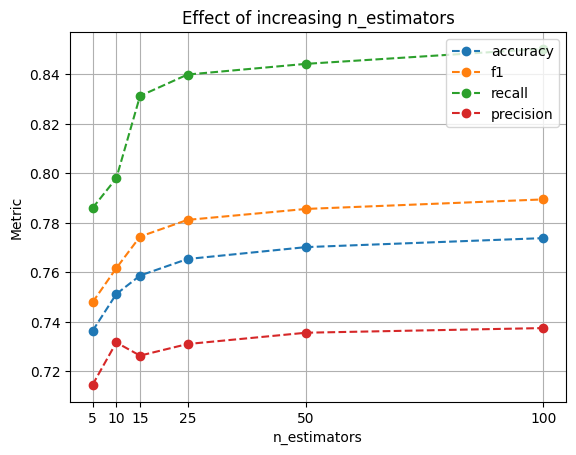
We can see that increasing n_estimators drives our metrics up; however, after 25 estimators, the improvements get increasingly small. Considering that a larger number of n_estimators will increase the runtime of each experiment, we can use this plot to inform our following experiments, cap n_estimators, and focus on other parameters.
In this blog post, we introduced a new experiment tracker that does not require any server running in the background or extra code and gives you the power of SQL to query and compare your experiments. Let us know what you think by opening an issue on the GitHub repository or sending us a message on Slack!
Seamless deployment for data scientists and developers. Ploomber handles infrastructure so you focus on building. Secure and scalable—from personal projects to enterprise apps. Support for Streamlit, Dash, Docker, and AI-powered applications. Because life's too short for deployment headaches.