


TL;DR; we forked
ipython-sql(pip install jupysql) and are actively developing it to bring a modern SQL experience to Jupyter! We’ve already built some great features, such as SQL query composition and plotting for large-scale datasets!
A few months after I started my career in Data Science, I encountered the ipython-sql package (which enables you to write cells like %sql SELECT * FROM table), and I was amazed by it. It allowed me to write SQL cells, making my notebooks much cleaner since I no longer needed to wrap each SQL query into a Python call. Furthermore, it also led me to learn that Jupyter (known as IPython back then) runs a modified Python interpreter, which enables all kinds of fun stuff like “magics” (e.g., %%bash, %%capture, etc.)
Fast forward, the Ploomber team has been busy helping dozens of companies use notebooks more effectively: from notebook profiling, unit testing, experiment tracking, and notebook deployment, we’ve seen hundreds of use cases. One of the most recurrent ones is SQL-heavy notebooks, used for scheduled reporting: a data practitioner writes some SQL in a notebook that produces some plots. Then, it is turned into a scheduled job to deliver results daily/weekly.
Many of those notebooks we’ve seen use the pandas.read_sql (or a variant of it) for running SQL queries. Whenever we saw this, we’d recommend a switch to ipython-sql, to simplify notebooks. However, in some cases, this would lead to some limitations and notebooks would end up with a mix of %%sql and pandas.read_sql calls. Since we love the %%sql abstraction, we decided to fork the repository and speed up development to bring the best of SQL to the notebooks world! We’re thankful to the original maintainers and contributors for such a great package.
We’ve released several new features already: better connection management, composing large SQL features, plotting large-scale datasets, among others. So let’s see what’s new!
We wrote this blog post in Jupyter (thanks to our Jupyblog package), so let’s start by installing and configuring a few things. We’ll be using DuckDB and the penguins dataset for the examples.
%pip install jupysql duckdb-engine --quiet
%load_ext sql
%config SqlMagic.displaylimit = 5
%sql duckdb://
Console output (1/1):
Note: you may need to restart the kernel to use updated packages.
from pathlib import Path
from urllib.request import urlretrieve

if not Path("penguins.csv").is_file():
    urlretrieve("https://raw.githubusercontent.com/mwaskom/seaborn-data/master/penguins.csv",
                "penguins.csv")
Great, we’re ready to start querying our data.
JupySQL is fully compatible with notebooks authored using ipython-sql; all arguments and configuration settings remain the same.
There is the usual line magic:
%sql SELECT * FROM penguins.csv LIMIT 3
Console output (1/2):
*  duckdb://
Done.
Console output (2/2):
| species | island | bill_length_mm | bill_depth_mm | flipper_length_mm | body_mass_g | sex |
|---|---|---|---|---|---|---|
| Adelie | Torgersen | 39.1 | 18.7 | 181 | 3750 | MALE |
| Adelie | Torgersen | 39.5 | 17.4 | 186 | 3800 | FEMALE |
| Adelie | Torgersen | 40.3 | 18.0 | 195 | 3250 | FEMALE |
And a cell magic:
%%sql
SELECT *
FROM penguins.csv
LIMIT 3
Console output (1/2):
*  duckdb://
Done.
Console output (2/2):
| species | island | bill_length_mm | bill_depth_mm | flipper_length_mm | body_mass_g | sex |
|---|---|---|---|---|---|---|
| Adelie | Torgersen | 39.1 | 18.7 | 181 | 3750 | MALE |
| Adelie | Torgersen | 39.5 | 17.4 | 186 | 3800 | FEMALE |
| Adelie | Torgersen | 40.3 | 18.0 | 195 | 3250 | FEMALE |
We improved support for managing multiple connections via a new --alias argument. Before that, users relied on the connection string to switch and close connections. Let’s create a new connection to an in-memory SQLite database:
%sql sqlite:// --alias second-db
We see the new connection is listed:
%sql
Console output (1/1):
duckdb://
*  (second-db) sqlite://
And we can close it using the alias:
%sql --close second-db
%sql
Console output (1/1):
duckdb://
A recurrent pattern we’ve seen is notebooks that use Jinja/templates for writing large queries (if you’re a dbt user, you know what I’m talking about). In JupySQL, you can write short queries, and we’ll automatically convert them into CTEs; let’s see an example and define a query that subsets our data:
%%sql duckdb:// --save adelie
SELECT *
FROM penguins.csv
WHERE species = 'Adelie'
Console output (1/2):
Done.
Console output (2/2):
| species | island | bill_length_mm | bill_depth_mm | flipper_length_mm | body_mass_g | sex |
|---|---|---|---|---|---|---|
| Adelie | Torgersen | 39.1 | 18.7 | 181 | 3750 | MALE |
| Adelie | Torgersen | 39.5 | 17.4 | 186 | 3800 | FEMALE |
| Adelie | Torgersen | 40.3 | 18.0 | 195 | 3250 | FEMALE |
| Adelie | Torgersen | None | None | None | None | None |
| Adelie | Torgersen | 36.7 | 19.3 | 193 | 3450 | FEMALE |
Now, let’s say that we want to build on top of the previous data subset; we could manually copy our last query and embed it in a new cell with a CTE, something like this:
WITH adelie AS (
    SELECT *
    FROM penguins.csv
    WHERE species = 'Adelie'
)

{your query here}
However, this has many problems:
To fix this, JupySQL brings a new --with argument that will automatically build the CTE for us:
%%sql --with adelie
SELECT *
FROM adelie
WHERE island = 'Torgersen'
Console output (1/2):
*  duckdb://
Done.
Console output (2/2):
| species | island | bill_length_mm | bill_depth_mm | flipper_length_mm | body_mass_g | sex |
|---|---|---|---|---|---|---|
| Adelie | Torgersen | 39.1 | 18.7 | 181 | 3750 | MALE |
| Adelie | Torgersen | 39.5 | 17.4 | 186 | 3800 | FEMALE |
| Adelie | Torgersen | 40.3 | 18.0 | 195 | 3250 | FEMALE |
| Adelie | Torgersen | None | None | None | None | None |
| Adelie | Torgersen | 36.7 | 19.3 | 193 | 3450 | FEMALE |
In the background, JupySQL runs the following:
WITH adelie AS (
    SELECT *
    FROM penguins.csv
    WHERE species = 'Adelie'
)

SELECT *
FROM adelie
WHERE island = 'Torgersen'
%sqlplotSQL notebooks almost always contain visualizations that allow data practitioners to understand their data. However, we saw two significant limitations when creating plots:
matplotlib (and seaborn) require all data to exist locally for plotting. This approach made notebooks extremely inefficient and incurred high data transfer costs.matplotlib would start accumulating intermediate results into memory.We created a new %sqlplot magic to fix this issue. %sqlplot performs most transformations in the SQL engine and only transfers the summary statistics required, drastically reducing data transfer and allowing practitioners to leverage the highly optimized SQL engines that data warehouses have. Furthermore, it enables them to plot larger-than-memory .csv and .parquet files via DuckDB. Let’s see an example.
First, let’s store a query that filters out NULLs:
%%sql --save not-nulls --no-execute
SELECT *
FROM penguins.csv
WHERE bill_length_mm IS NOT NULL
AND bill_depth_mm IS NOT NULL
Console output (1/1):
*  duckdb://
Skipping execution...
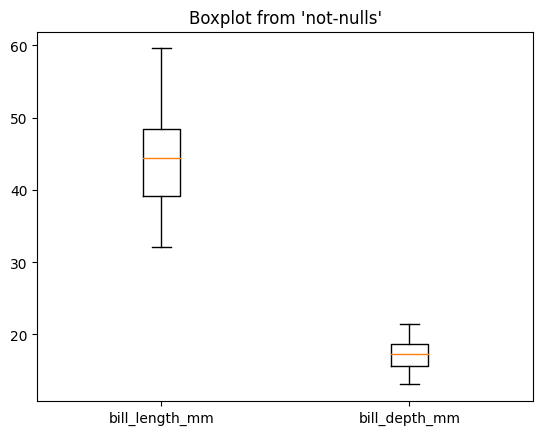
Now, we create a boxplot. A boxplot requires computing percentiles and a few other statistics. Those are all computed in the SQL engine (in this case, DuckDB). Then we use those statistics to create the plot:
%sqlplot boxplot --column bill_length_mm bill_depth_mm --table not-nulls --with not-nulls
Console output (1/1):
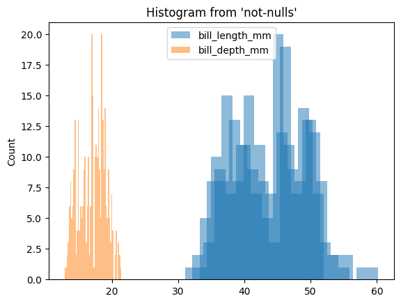
We can also create a histogram. All the data is aggregated in DuckDB (or the data warehouse), and only the bins and counts are retrieved:
%sqlplot histogram --column bill_length_mm bill_depth_mm --table not-nulls --with not-nulls
Console output (1/1):
Often, users want to customize database connections to bring extra features. ipython-sql only allows establishing connections via a connection string, severely limiting adoption. In JupySQL, you may pass existing connections. Let me show you two example use cases.
If using DuckDB, you can create a connection, register existing data frames, pass the customized engine, and query them with SQL:
import pandas as pd
from sqlalchemy import create_engine

engine = create_engine("duckdb:///:memory:")
engine.execute("register", ("df", pd.DataFrame({"x": range(100)})))
Console output (1/1):
<sqlalchemy.engine.cursor.LegacyCursorResult at 0x11ddbd9a0>
%sql engine
%%sql
SELECT *
FROM df
WHERE x > 95
Console output (1/2):
duckdb://
*  duckdb:///:memory:
Done.
Console output (2/2):
| x |
|---|
| 96 |
| 97 |
| 98 |
| 99 |
If using SQLite, passing a custom connection allows you to register user-defined functions (UDFs):
from sqlalchemy import create_engine
from sqlalchemy import event

def mysum(x, y):
    return x + y

engine_sqlite = create_engine("sqlite://")

@event.listens_for(engine_sqlite, "connect")
def connect(conn, rec):
    conn.create_function(name="MYSUM", narg=2, func=mysum)
%sql engine_sqlite
%%sql
SELECT MYSUM(1, 2)
Console output (1/2):
duckdb://
   duckdb:///:memory:
*  sqlite://
Done.
Console output (2/2):
| MYSUM(1, 2) |
|---|
| 3 |
We’ve completely revamped the documentation using Jupyter Book and following the documentation system. You can find a Quick Start section, a detailed User Guide, and the technical API reference. Furthermore, all our tutorials contain a 🚀 button that will start a temporary JupyterLab session for you to try it out!
We’re stoked to be working on JupySQL. Its user base has been growing rapidly, cementing our conviction that the data community wants a better SQL experience in Jupyter. There are a few things we’re working on, and we’ll release soon, so stay tuned (we’re on Twitter and LinkedIn). If you want to share your feedback, feel free to open an issue on GitHub or send us a message on Slack!
Seamless deployment for data scientists and developers. Ploomber handles infrastructure so you focus on building. Secure and scalable—from personal projects to enterprise apps. Support for Streamlit, Dash, Docker, and AI-powered applications. Because life's too short for deployment headaches.