Introduction to Logistic Regression

There are different models and algorithms for classification problems. Logistic regression is a very efficient model especially when we talk about binary classification. In this post, we share with you what’s behind the logistic regression algorithm, and how you can perform it with a sample dataset. Code is provided!

What is logistic regression?

Logistic regression is a supervised learning algorithm, which is mainly used for binary classification tasks. Customer churn and spam email detection are typical problems for which logistic regression offers an efficient and practical solution.

Logistic regression algorithm is based on the logistic function (i.e. sigmoid function) so it’s better to start with learning this function.

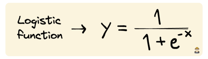
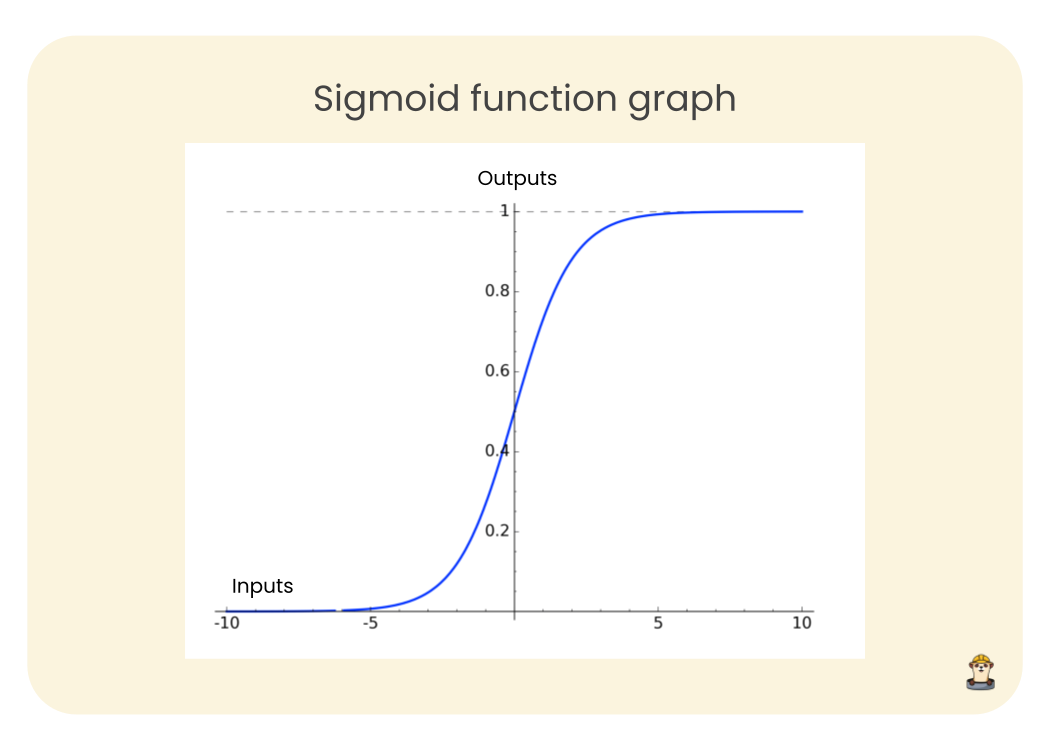
What the logistic function does is take any real-valued number as input and map it to a value between 0 and 1. Thus, whatever the input value is, the output will be between 0 and 1. The following image shows the plot of the logistic function.

To better understand how logistic function is used in the logistic regression algorithm, let’s show it in a different way:

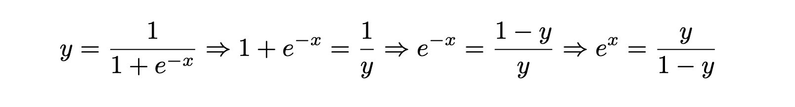
Taking the natural log of both sides:

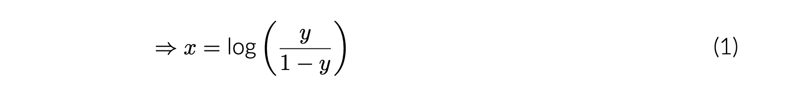
In the case of the logistic regression algorithm, the input x becomes a linear equation formed by the features in the dataset. The output y is a probability value. For instance, an output of 0.7 means that there is a 70% chance that this data point (i.e. observation) belongs to the positive class.

When y is a probability value, then the expression in the right hand side of the equation (1) above is called log odds, a term used in probability. Log odds of probability 0.5 is 0. Thus, if we solve the linear equation for 0, we find the solution for which the probability of the observation belonging to the positive class is 0.5. For the positive output values, the probability of the positive class is more than 0.5 and for the negative output values, the probability of the positive class is less than 0.5

This is how the logistic regression algorithm works. In a sense, it solves a linear equation to perform a binary classification task.

Creating a logistic regression model with Scikit-learn

We will try to solve a customer churn problem with a logistic regression model. The dataset is called Telco Customer Churn and it is available on Kaggle. This dataset contains a lot of features that define the demographics and shopping behaviors of customers.

Once the dataset has been downloaded, we will rename it to telco_customer_churn.csv for simplicity.

After an initial exploratory data analysis, we decide to drop some of the features that won’t be relevant to our customer churn regression example.

import pandas as pd


df = pd.read_csv("telco_customer_churn.csv")
df.drop([
    "customerID", "gender", "PhoneService", "Contract",
    "TotalCharges", "StreamingTV", "StreamingMovies"
], axis=1, inplace=True)

df.head()

Data preprocessing

The dataset needs a bit of data preprocessing. We will first encode the categorical variables, which can be done using the get_dummies function of Pandas.

After applying the function, we can verify that the dataframe has been encoded:

cat_features = [
    'SeniorCitizen', 'Partner', 'Dependents', 'MultipleLines',
    'InternetService','OnlineSecurity', 'OnlineBackup', 'Churn',
    'DeviceProtection', 'TechSupport', 'PaperlessBilling',
    'PaymentMethod'
]

df = pd.concat([
    pd.get_dummies(df[cat_features], drop_first=True),
    df[["tenure", "MonthlyCharges"]]
], axis=1)

df = df.rename(columns = {"Churn_Yes": "Churn"})

df.head()

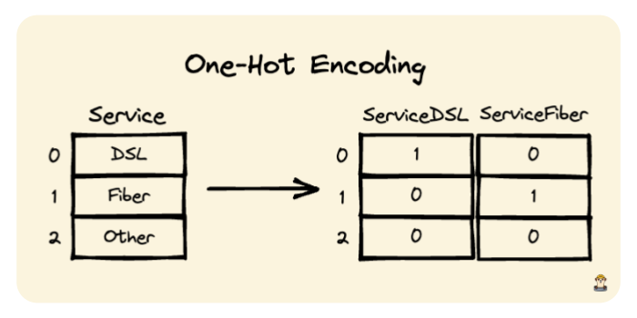
What we have done using the get_dummies function is called one-hot encoding. When used with the drop_first parameter set as True, it converts binary columns (e.g. Yes and No) to a column with 1 and 0 values. If a column has 3 different values, then it works as shown in the drawing below:

Model creation

The next step is to split the data into train and test sets, which can be done using the train_test_split function from scikit-learn.

For reproducibility of this post, we will fix the random seed using numpy, so you are able to get the same results of the experiment.

from sklearn.model_selection import train_test_split
import numpy as np


# We fix the random seed
np.random.seed(321)

X = df.drop("Churn", axis=1)
y = df["Churn"]

X_train, X_test, y_train, y_test = train_test_split(
    X, y, test_size=0.25
)

X contains the features and y is the target variable.

Another part of data preprocessing for this dataset is normalizing the numerical features. We need to make the value ranges of different features similar. Otherwise, variables with higher values will be given more importance which affects the accuracy of the model. One option for normalizing is using the min-max scaler, which brings all the values into the range of 0-1.

The maximum and minimum values will be changed to 1 and 0, respectively. All other values are in between.

from sklearn.preprocessing import MinMaxScaler


scaler = MinMaxScaler()
scaler.fit(X_train[["tenure", "MonthlyCharges"]])

X_train[["tenure", "MonthlyCharges"]] = \
scaler.transform(X_train[["tenure", "MonthlyCharges"]])

X_test[["tenure", "MonthlyCharges"]] = \
scaler.transform(X_test[["tenure", "MonthlyCharges"]])

The first step is to create a scaler object, which is trained with the features in the train set. Then, it is used for transforming features in both the train and test sets.

We are now ready to create a model and train it. We will create a logistic regression model available in the linear_model module of scikit-learn. Then, the model will be trained using the train set. Finally, we will make predictions on both the train and test sets and measure the accuracy.

from sklearn.linear_model import LogisticRegression
from sklearn.metrics import accuracy_score


clf = LogisticRegression()
clf.fit(X_train, y_train)

y_train_predict = clf.predict(X_train)
y_test_predict = clf.predict(X_test)

accuracy_train = accuracy_score(y_train, y_train_predict)
accuracy_test = accuracy_score(y_test, y_test_predict)

print("Training accuracy:", accuracy_train)
print("Testing accuracy:", accuracy_test)

The trained model achieves an accuracy around 0.8 on both train and test sets. However, accuracy is not always the best metric to evaluate the performance of a classification model especially when the target variable is unbalanced as in the customer churn and spam email detection tasks.

For instance, we might be interested in how many of the churned customers are detected by the model. We can use a confusion matrix to see a more detailed overview of the predictions. The sklearn-evaluation library can be used for visualizing the confusion matrix.

import matplotlib.pyplot as plt
from sklearn_evaluation import plot


print("Let's see the number of churns in testing dataset:")
print(y_test.value_counts())

plt.figure(figsize=(7,5))
plot.confusion_matrix(y_test, y_test_predict)
plt.show()

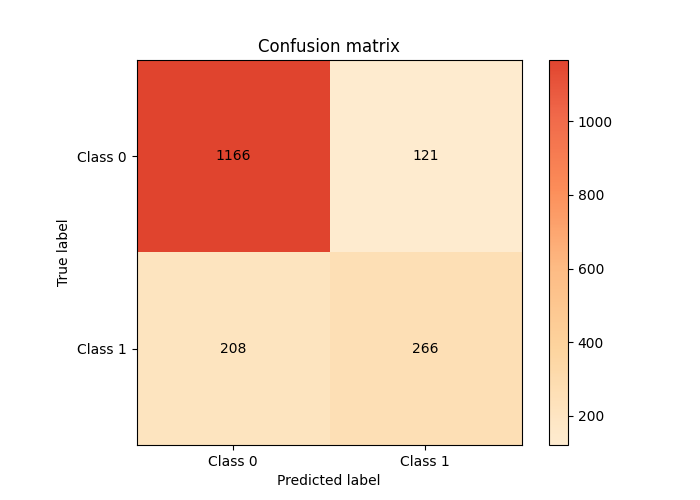
The model was able to predict 266 of 474 churned customers. This is not a very good performance if our focus is to catch customers who are likely to churn.

We can use the class_weight parameter to improve the performance of the model on the positive class. Let’s create a new logistic regression model using this parameter.

clf_improved = LogisticRegression(class_weight={0: 1, 1: 3})
clf_improved.fit(X_train, y_train)

y_train_predict_improved = clf_improved.predict(X_train)
y_test_predict_improved = clf_improved.predict(X_test)

accuracy_train_improved = accuracy_score(y_train, y_train_predict_improved)
accuracy_test_improved = accuracy_score(y_test, y_test_predict_improved)

print("Training accuracy (improved):", accuracy_train_improved)
print("Testing accuracy (improved):", accuracy_test_improved)

Now, if we use sklearn-evaluation again to plot the new confusion matrix:

plt.figure(figsize=(7,5))
plot.confusion_matrix(y_test, y_test_predict)
#plt.show()
plt.savefig("plot.png")

The weights assigned to negative (not churned) and positive (churned) classes are 1 and 3, respectively. After repeating the training and making predictions and plotted the confusion matrix of this improved model, we can see how it is different from the previous one.

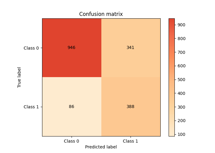
The second model was able to predict 388 of 474 churned customers, which is much better than the previous model. However, the overall accuracy has dropped to 0.75 on the test set. We sacrifice the predictions on the negative class for being able to increase the correct predictions on the churned customers.

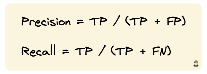
The metric we focused on in the second model is called precision, which measures how good our model is when the prediction is positive. To calculate precision, the number of correct positive predictions is divided by the number of all positive predictions.

Another commonly used metric in classification problems is recall, which measures how good our model is at correctly predicting positive classes. To calculate precision, the number of correct positive predictions is divided by the number of all positive examples.

• True positive (TP): Both the prediction and actual value is positive
• False positive (FP): Prediction is positive but the actual value is negative
• True negative (TN): Both the prediction and actual value is negative
• False negative (FN): Prediction is negative but the actual value is positive

Conclusion

Logistic regression is a very efficient model especially in binary classification problems. It is not as flexible as complex algorithms such as random forests. However, it is easy to implement and interpret. Thus, it’s definitely worth a try.

Another advantage of logistic regression is that we can use the probability output as is which allows us to set a threshold when creating binary outputs. For instance, we can make a logistic regression model predict positive only if the probability of positive class is more than 0.8. This feature comes in handy for some tasks where we need to be more certain when predicting the positive class.