


We presented a shorter version of this blog series at PyData Global 2021.
Click here for Part I, here for Part III.
In this series’s first part, we started with a simple smoke testing strategy to ensure our code runs on every git push. Then, we built on top of it to ensure that our feature generation pipeline produced data with a minimum level of quality (integration tests) and verified the correctness of our data transformations (unit tests).
Now, we’ll add more robust tests: distribution changes, ensure that our training and serving logic is consistent, and check that our pipeline produces high-quality models.
If you’d like to know when the third part is out, subscribe to our newsletter, follow us on Twitter or LinkedIn.
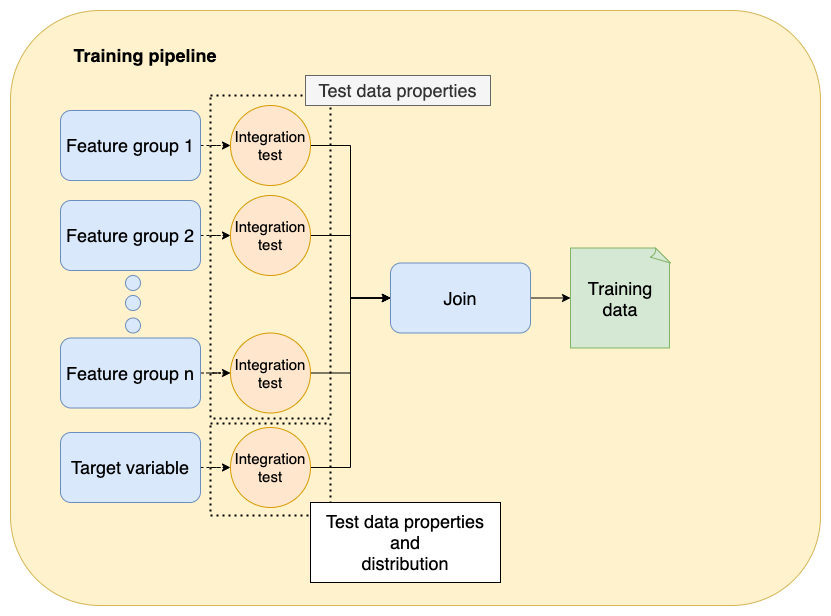
In the previous level, we introduced integration testing to check our assumptions about the data. Such tests verify basic data properties such as no NULLs, or numeric ranges. However, if working on a supervised learning problem, we must take extra care of the target variable and check its distribution to ensure we don’t train on incorrect data. Let’s see an example.
In a previous project, I needed to update my training set with new data. After doing so and training a new model, the evaluation metrics improved a lot. I was skeptical but couldn’t find any issues in recent code changes. So I pulled out the evaluation report from the model in production and compared it with the one I had trained. The evaluation report included a table with a training data summary: the mean of the target variable had reduced drastically:
| Statistic | Old training data | New training data |
|---|---|---|
| Mean | 10 | 5 |
| Standard deviation | 2 | 1 |
Since the mean of the target variable decreased, the regression problem got easier. Picture the distribution of a numerical variable: a model predicting zero will have an MAE equal to the absolute mean of the distribution; now, imagine you add recently generated data that increases the concentration of your target variable even more (i.e., the mean decreases): if you evaluate the model that always predicts zero, the MAE will decrease, giving the impression that your new model got better!
After meeting with business stakeholders, we found out that a recent change in the data source introduced spurious observations. After such an incident, I created a new integration test that compared the mean and standard deviation of the target variable to a reference value (obtained from the training set used by the current production model):
def test_target_variable(df_training):
    # get mean and std for current training set
    y_mean = df_training.y.mean()
    y_std = df_training.y.std()

    # load reference values (e.g., from a database)
    y_mean_lower_ref, y_mean_upper_ref = load_y_mean_ref()
    y_std_lower_ref, y_std_upper_ref = load_y_std_ref()

    # stop execution if mean or std are outside the boundaries
    assert y_mean_lower_ref <= y_mean <= y_mean_upper_ref
    assert y_std_lower_ref <= y_std <= y_std_upper_ref
Don’t overthink the reference values; take your previous values and add some tolerance. Then, if the test fails, investigate if it’s due to a fundamental change in the data generation process (in such a case, you may want to update your reference values) and not due to some data error. If you’re working on a classification problem instead, you can compare the proportion of each label.
We could apply the same logic to all features and test their distributions: since they shouldn’t change drastically from one commit to the next. However, manually computing the reference ranges will take a lot of time if you have hundreds of features, so at the very least, test the distribution of your target variable.
Note that comparing mean and standard deviation is a simple (but naive) test, it works well if you don’t expect your data to change much from one iteration to the next one, but a more robust and statisically principled way of comparing distributions is the KS test. Here’s a sample KS test implementation.
Deploying a model involves a few more steps than loading a .pickle file and calling model.predict(some_input). You most likely have to preprocess input data before passing it to the model. More importantly, you must ensure that such preprocessing steps always happen before calling the model. To achieve this, encapsulate inference logic in a single call:
from myproject import ServingPipeline

pipeline = ServingPipeline()
prediction = pipeline.predict(data=some_input_data)
Once you encapsulate inference logic, ensure you throw an error on invalid input data. Raising an exception protects against ill-defined cases (it’s up to you to define them). For example, if you’re expecting a column containing a price quantity, you may raise an error if it has a negative value.
There could be other cases where you do not want your model to make a prediction. For example, you may raise an error when the model’s input is within a subpopulation where you know the model isn’t accurate.
The following sample code shows how to test exceptions in pytest:
import pytest

from myproject import ServingPipeline

def test_error_on_invalid_data():
    some_invalid_data = {
        'price': -10
    }

    pipeline = ServingPipeline()

    with pytest.raises(ValueError) as excinfo:
        pipeline.predict(data=some_invalid_data)
The example above is a new type of unit test; instead of checking that something returns a specific output, we test that it raises an error. Inside your ServingPipeline.predict method, you may have something like this:
# ServingPipeline.py

# is_valid contains logic to validate input data
from my_project import is_valid

class ServingPipeline:
    # ...
    # ...

    def predict(self, data):
        if data['price'] < 0:
            raise ValueError('Price must be a positive value')
To learn more about testing exceptions with pytest, click here.
Here’s a sample implementation that checks that our pipeline throws a meaningful error when passed incorrect input data.
At this level, we test that our inference pipeline is correct. We must verify two aspects to assess the correctness of our inference pipeline:
Training-serving skew is one of the most common problems in ML projects. It happens when the input data is preprocessed differently at serving time (compared to training time). Ideally, we should share the same preprocessing code at serving and training time; however, even if that’s the case, it’s still essential to check that our training and serving code preprocess the data in the same manner.
The test is as follows: sample some observations from your raw data and pass them through your data processing pipeline to obtain a set of (raw_input, feature_vector) pairs. Now, take the same inputs, pass them through your inference pipeline, and ensure that both feature vectors match precisely.
from my_project import sample_observations_and_generate_features, ServingPipeline

def test_training_serving_skew():
    # assume this is captures the logic in your training pipeline
    input_raw, feature_vector = sample_observations_and_generate_features()
    inference = ServingPipeline()
    # assume ServingPipeline.generate_features generates the feature vector
    # using your serving logic
    fewature_vector_serving = inference.generate_features(input_raw)
    assert feature_vector == feature_vector_serving
Here’s a sample implementation of a test from our sample repository that checks there is no training-serving skew.
To simplify maintaining a training and serving pipeline, check out Ploomber, one of our features is to transform batch-based training pipeline into an in-memory one without code changes.
Imagine I deployed a model that used ten features a month ago. Now, I’m working on a new one, so I add the corresponding code to the training pipeline and deploy: production breaks. What happened? I forgot to update my inference pipeline to include the recently added feature. So, it’s essential to add another test to ensure your inference code correctly integrates with the model file produced by the training pipeline: the inference pipeline should generate the same features that the model was trained on.
from my_project import sample_observations_and_generate_features, ServingPipeline

def test_inference_pipeline_integration():
    # assume this is the logic in your training pipeline
    input_raw, feature_vector = sample_observations_and_generate_features()
    inference = ServingPipeline()
    # ensure that you can generate predictions from raw data
    assert inference.predict(input_raw)
In our sample project, we first train a model with a sample of the data, then we ensure that we can use the trained model to generate predictions. Such a test is implemented in the ci.yml file, and it executes on each git push.
Before deploying a model, it’s essential to evaluate it offline to ensure that it has at least the same performance as a benchmark model. A benchmark model is often the current model in production. This model quality test helps you quickly ensure that releasing some candidate model to production is acceptable.
For example, if you’re working on a regression problem and use Mean Absolute Error (MAE) as your metric, you may compute MAE across the validation set and for some sub-populations of interest. Say you deployed a model and calculated your MAE metrics; after some work, you added a new feature to improve model metrics. Finally, you train a new model and generate metrics:
| Validation set | Benchmark MAE | Candidate model MAE |
|---|---|---|
| Complete | 1.4 | 1.2 |
| Sub-population 1 | 0.5 | 0.4 |
| Sub-population 2 | 2.0 | 2.1 |
How do you compare these results? At first glance, it looks like your model is working because it reduced MAE for the first two metrics, although it increased them in the third group. Is this model better?
It’s hard to judge based on a single set of reference values. So instead of having a single set of reference values, create a distribution by training the production model with the same parameters multiple times. Say we repeat our training procedure three times for the benchmark model and the candidate model, and we get three data points this time:
| Validation set | Benchmark MAE | Candidate model MAE |
|---|---|---|
| Complete | 1.4, 1.2, 1.3 | 1.2, 1.1, 1.2 |
| Sub-population 1 | 0.5, 0.5, 0.6 | 0.4, 0.4, 0.3 |
| Sub-population 2 | 2.0, 2.3, 2.4 | 2.1, 2.0, 2 |
We now have an empirical distribution. Then you can compare that the metrics in your candidate model are within the observed range:
def test_expected_metrics():
    # load reference min/max values (e.g., from a database)
    lower_ref, upper_ref = load_reference()
    current = load_current()
    assert lower_ref <= current <= upper_ref
Here’s a test implementation in our sample repository.
Note that we’re evaluating current on both sides; this is essential because we want the tests to alert us when our model drops in performance and increases steeply. While performance increases are great news, we should make sure that such increase is due to some specific improvement (e.g., training on more data, adding new features) and not due to a methodological error such as information leakage.
Note: Evaluating model performance with minimum and maximum metric values is a simple way to get started, however, at some point you may want to implement more statistically principled approaches, this article reviews a few methods for doing so.
It is critical to test model quality on every code change. For example, imagine you haven’t run your tests in a while; since the last time you ran them, you increased the training set size, added more features, and optimized the performance of some data transformations. You then train a model, and the test breaks because the pipeline produced a model with higher performance. In such a case, you may need to train models from previous commits to know what action caused the model’s performance to fall out of the expected range. Compare that to the scenario where you test on each change: if your model increases performance when adding more training data, that’s great news! But if you improved the performance (i.e., to use less memory) of some data transformation and your model is better all of a sudden, there’s reason to be skeptical.
From a statistical perspective, the more metrics to compare, the higher the chance of your test to fail. A test that fails with no apparent reason isn’t great. To increase the reliability of such a test, you have two options:
For critical models, it’s a good idea to complement the previous model quality testing with some manual quality assessment. Manual assessment helps because some model properties are more difficult to test automatically but show up quickly by visual human inspection; once you detect any critical metrics to track, you can include them in the automated test.
One way to quickly generate model evaluation reports is to run your training code as a notebook; for example, say your train.py script looks like this:
from sklearn.ensemble import RandomForestRegressor
# assume the function "evaluate" creates evaluation charts and tables
from my_project import load_training_data, evaluate

X_train, y_train = load_training_data()

model = RandomForestRegressor()
model.fit(X_train, y_train)

# returns a matplotlib figure
evaluate.plot_pred_vs_actual(y_pred, y_train)

# returns a data frame with metrics across sub-populations
evaluate.metrics_table(X, y_pred, y_train)
Instead of writing extra code to save the chart and the table in a .html file, you can use Ploomber, which automatically converts your .py to .ipynb (or .html) files at runtime, so you easily get a model evaluation report each time you train a new model. You can also use sklearn-evaluation which can compare multiple .ipynb files (see this example).
In this second part, we increase the robustness of our tests: we check for distribution changes in our target variable, ensure that our training and serving logic is consistent, and check that our pipeline produces high-quality models, concluding our 5-level framework.
In the following (and last) part of the series, we’ll provide extra advice to set up a streamlined workflow that allows us to repeat the develop -> test -> improve loop: we modify our pipeline, ensure that it works correctly, and continue improving.
If you’d like to know when the third part is out, subscribe to our newsletter, follow us on Twitter or LinkedIn.
Seamless deployment for data scientists and developers. Ploomber handles infrastructure so you focus on building. Secure and scalable—from personal projects to enterprise apps. Support for Streamlit, Dash, Docker, and AI-powered applications. Because life's too short for deployment headaches.