


In this blog post, I’ll show you how you can export your MLFlow data to a SQLite database so you can easily filter, search and aggregate all your Machine Learning experiments with SQL.
Note: You can get this post in notebook format from here.
MLFlow is one of the most widely used tools for experiment tracking, yet, its features for comparing experiments are severely limited. One basic operation I do with my Machine Learning experiments is to put plots side by side (e.g., confusion matrices or ROC curves); this simple operation isn’t possible in MLFlow (the issue has been open since April 2020).
Another critical limitation are its filtering and search capabilities. MLFlow defines its own filter DSL which is a limited version of a SQL WHERE clause. Even though MLFlow supports several SQL databases as backend, you have to use this limited DSL which only allows basic filtering but does not support aggregation or any other operation that you can trivially do with some lines of SQL. For me, this is a major drawback since often I want to perform more than a basic filter.
So let’s see how we can get our data out of MLFlow and into a SQLite database so we can easily explore our Machine Learning experiments! Under the hood, this will use the SQLiteTracker from the sklearn-evaluation package.
The code is in a Python package that you can install with pip:
pip install mlflow2sql
If you don’t have some sample MLFlow data, I wrote some utility functions to generate a few experiments and log them. However, you need to install a few extra dependencies:
pip install "mlflow2sql[demo]"
If you’re running this from a notebook, you can run the following cel to install the dependencies:
%pip install "mlflow2sql[demo]" --quiet
Console output (1/1):
Note: you may need to restart the kernel to use updated packages.
You can download some sample MLFlow data from here. Alternatively, you can generate it by running the following in a Python session (this will create the data in the ./mlflow-data directory):
import shutil
from pathlib import Path

from mlflow2sql import generate, export, ml

# clean up the directory, if any
path = Path("mlflow-data")
if path.exists():
    shutil.rmtree(path)

# generate sample data - takes a few minutes
with generate.start_mlflow(backend_store_uri="mlflow-data",
                           default_artifact_root="mlflow-data"):
    ml.run_default()
Console output (1/3):
[2022-12-21 14:28:49 -0600] [31007] [INFO] Starting gunicorn 20.1.0
[2022-12-21 14:28:49 -0600] [31007] [INFO] Listening at: http://127.0.0.1:5000 (31007)
[2022-12-21 14:28:49 -0600] [31007] [INFO] Using worker: sync
[2022-12-21 14:28:49 -0600] [31009] [INFO] Booting worker with pid: 31009
[2022-12-21 14:28:49 -0600] [31010] [INFO] Booting worker with pid: 31010
[2022-12-21 14:28:49 -0600] [31011] [INFO] Booting worker with pid: 31011
[2022-12-21 14:28:49 -0600] [31012] [INFO] Booting worker with pid: 31012
Console output (2/3):
Training GradientBoostingClassifier...
Executed 10/30 so far...
Executed 20/30 so far...
Executed 30/30 so far...
Training SVC...
Executed 10/12 so far...
Training RandomForestClassifier...
Executed 10/54 so far...
Executed 20/54 so far...
Executed 30/54 so far...
Executed 40/54 so far...
Executed 50/54 so far...
Console output (3/3):
[2022-12-21 14:32:29 -0600] [31007] [INFO] Handling signal: term
[2022-12-21 14:32:29 -0600] [31010] [INFO] Worker exiting (pid: 31010)
[2022-12-21 14:32:29 -0600] [31011] [INFO] Worker exiting (pid: 31011)
[2022-12-21 14:32:29 -0600] [31009] [INFO] Worker exiting (pid: 31009)
[2022-12-21 14:32:29 -0600] [31012] [INFO] Worker exiting (pid: 31012)
[2022-12-21 14:32:30 -0600] [31007] [INFO] Shutting down: Master
Once you have some MLFlow data, start a Python session, define the BACKEND_STORE_URI and DEFAULT_ARTIFACT_ROOT variables in the next code snippet.
Note that the two variables correspond to the two arguments with the same name that you pass when starting the MLFlow server:
mlflow server --backend-store-uri BACKEND_STORE_URI --default-artifact-root DEFAULT_ARTIFACT_ROOT
Note: If you didn’t pass those arguments when running mlflow server, the default value is ./mlruns.
from mlflow2sql import export, ml

# these two variables are ./mlruns by default
BACKEND_STORE_URI = "mlflow-data"
DEFAULT_ARTIFACT_ROOT = "mlflow-data"

# note: this was tested with MLFlow versions 1.30.0 and 2.0.1
runs = export.find_runs(backend_store_uri=BACKEND_STORE_URI,
                        default_artifact_root=DEFAULT_ARTIFACT_ROOT)
We can get the number of experiments we extracted:
len(runs)
Console output (1/1):
96
Let’s now initialize our experiment tracker (documentation available here), and insert our MLFlow experiments:
from sklearn_evaluation import SQLiteTracker

# clean up the database, if any
db = Path("experiments.db")

if db.exists():
    db.unlink()

tracker = SQLiteTracker('experiments.db')
tracker.insert_many((run.to_dict() for run in runs))
Let’s check the number of extracted experiments:
len(tracker)
Console output (1/1):
96
Great! We got all of them in the database. Let’s start exploring them with SQL!
SQLiteTracker creates a table with all our experiments and it stores the logged data in a JSON object with three keys: metrics, params, and artifacts:
tracker.query("""
SELECT
    uuid,
    json_extract(parameters, '$.metrics') as metrics,
    json_extract(parameters, '$.params') as params,
    json_extract(parameters, '$.artifacts') as artifacts
    FROM experiments
LIMIT 3
""")
Console output (1/1):
| metrics | params | artifacts | |
|---|---|---|---|
| uuid | |||
| 42dc4d08 | {"recall":[["1671654737960"],["0.8666260657734... | {"max_depth":10,"model_name":"RandomForestClas... | {"confusion_matrix_png":"<img src=\"data:image... |
| 9cef8649 | {"recall":[["1671654632100"],["0.8331303288672... | {"probability":true,"model_name":"SVC","C":2.0... | {"confusion_matrix_png":"<img src=\"data:image... |
| 053f4f97 | {"recall":[["1671654699203"],["0.8623629719853... | {"max_depth":10,"model_name":"RandomForestClas... | {"confusion_matrix_png":"<img src=\"data:image... |
We can extract the metrics easily. Note that MLFlow stores metrics in the following format:
(timestamp 1) (value 1)
(timestamp 2) (value 2)
Hence, when parsing it, we create two lists. One with the timestamps and another one with the values:
[[ts1, ts2], [val1, val2]]
Let’s extract the metrics values and sort by F1 score, note that .query() returns a pandas.DataFrame by default:
tracker.query("""
SELECT
    uuid,
    json_extract(parameters, '$.metrics.f1[1][0]') as f1,
    json_extract(parameters, '$.metrics.precision[1][0]') as precision,
    json_extract(parameters, '$.metrics.recall[1][0]') as recall,
    json_extract(parameters, '$.params.model_name') as model_name
FROM experiments
ORDER BY f1 DESC
LIMIT 10
""")
Console output (1/1):
| f1 | precision | recall | model_name | |
|---|---|---|---|---|
| uuid | ||||
| 1fb0cd23 | 0.8040023543260741 | 0.7779043280182233 | 0.8319123020706456 | RandomForestClassifier |
| 07043ccb | 0.8032883147386964 | 0.7755102040816326 | 0.833130328867235 | RandomForestClassifier |
| b9a0c264 | 0.802570093457944 | 0.7710437710437711 | 0.8367844092570037 | RandomForestClassifier |
| 9dfec05b | 0.8018675226145316 | 0.7697478991596639 | 0.8367844092570037 | RandomForestClassifier |
| d14170de | 0.8013998250218723 | 0.7688864017907107 | 0.8367844092570037 | RandomForestClassifier |
| 3da71d72 | 0.8005856515373354 | 0.7710095882684715 | 0.8325213154689404 | RandomForestClassifier |
| cdccf858 | 0.7994358251057828 | 0.744613767735155 | 0.8629719853836785 | RandomForestClassifier |
| 461ec80d | 0.7987475092513522 | 0.7498663816141101 | 0.8544457978075518 | RandomForestClassifier |
| 9cef8649 | 0.7981330221703616 | 0.7659574468085106 | 0.833130328867235 | SVC |
| db59ecf8 | 0.7978817299205649 | 0.771770062606716 | 0.8258221680876979 | RandomForestClassifier |
We can also extract the artifacts and display them inline by passing as_frame=False and render_plots=True:
results = tracker.query("""
SELECT
    uuid,
    json_extract(parameters, '$.metrics.f1[1][0]') as f1,
    json_extract(parameters, '$.params.model_name') as model_name,
    json_extract(parameters, '$.metrics.precision[1][0]') as precision,
    json_extract(parameters, '$.metrics.recall[1][0]') as recall,
    json_extract(parameters, '$.artifacts.confusion_matrix_png') as confusion_matrix,
    json_extract(parameters, '$.artifacts.precision_recall_png') as precision_recall
FROM experiments
ORDER BY f1 DESC
LIMIT 2
""", as_frame=False, render_plots=True)

results
Console output (1/1):
| uuid | f1 | model_name | precision | recall | confusion_matrix | precision_recall |
|---|---|---|---|---|---|---|
| 1fb0cd23 | 0.8040023543260741 | RandomForestClassifier | 0.7779043280182233 | 0.8319123020706456 |  |  |
| 07043ccb | 0.8032883147386964 | RandomForestClassifier | 0.7755102040816326 | 0.833130328867235 |  |  |
Looking at the plots is a bit difficult in the table view, but we can zoom in and extract them. Let’s get a tab view from our top two experiments. Here are the confusion matrices:
results.get("confusion_matrix")
Console output (1/1):
And here’s the precision-recall curve:
results.get("precision_recall")
Console output (1/1):
In our generated experiments, we trained some Support Vector Machines, Gradient Boosting and Random Forest. Let’s filter by Random Forest, sort by F1 score and extract their parameters. We can easily do this with SQL!
tracker.query("""
SELECT
    uuid,
    json_extract(parameters, '$.metrics.f1[1][0]') as f1,
    json_extract(parameters, '$.params.model_name') as model_name,
    json_extract(parameters, '$.metrics.precision[1][0]') as precision,
    json_extract(parameters, '$.metrics.recall[1][0]') as recall,
    json_extract(parameters, '$.params.max_depth') as max_depth,
    json_extract(parameters, '$.params.n_estimators') as n_estimators,
    json_extract(parameters, '$.params.criterion') as criterion
FROM experiments
WHERE model_name = 'RandomForestClassifier'
ORDER BY f1 DESC
LIMIT 3
""", as_frame=False, render_plots=True)
Console output (1/1):
| uuid | f1 | model_name | precision | recall | max_depth | n_estimators | criterion |
|---|---|---|---|---|---|---|---|
| 1fb0cd23 | 0.8040023543260741 | RandomForestClassifier | 0.7779043280182233 | 0.8319123020706456 | None | 50 | gini |
| 07043ccb | 0.8032883147386964 | RandomForestClassifier | 0.7755102040816326 | 0.833130328867235 | None | 50 | log_loss |
| b9a0c264 | 0.802570093457944 | RandomForestClassifier | 0.7710437710437711 | 0.8367844092570037 | None | 100 | entropy |
Finally, let’s do something a bit more sophisticated. Let’s get all the Random Forests, group by number of trees (n_estimators), and take the mean of our metrics. This will allow us to see what’s the effect of increasing the number of trees in the model’s perfomance:
df = tracker.query(
    """
SELECT
    json_extract(parameters, '$.params.n_estimators') as n_estimators,
    AVG(json_extract(parameters, '$.metrics.precision[1][0]')) as precision,
    AVG(json_extract(parameters, '$.metrics.recall[1][0]')) as recall,
    AVG(json_extract(parameters, '$.metrics.f1[1][0]')) as f1
FROM experiments
WHERE json_extract(parameters, '$.params.model_name') = 'RandomForestClassifier'
GROUP BY n_estimators
""",
    as_frame=True,
).set_index("n_estimators")

df
Console output (1/1):
| precision | recall | f1 | |
|---|---|---|---|
| n_estimators | |||
| 5 | 0.712230 | 0.793071 | 0.749882 |
| 10 | 0.731649 | 0.792191 | 0.759146 |
| 15 | 0.727118 | 0.826228 | 0.772904 |
| 25 | 0.734089 | 0.841318 | 0.783521 |
| 50 | 0.738559 | 0.846461 | 0.788263 |
| 100 | 0.735830 | 0.849303 | 0.788023 |
import matplotlib.pyplot as plt

fig, ax = plt.subplots()

for metric in ["f1", "recall", "precision"]:
    df[metric].plot(ax=ax, marker="o", style="--")

ax.legend()
ax.grid()
ax.set_title("Effect of increasing n_estimators")
ax.set_ylabel("Metric")
_ = ax.set_xticks(df.index)
Console output (1/1):
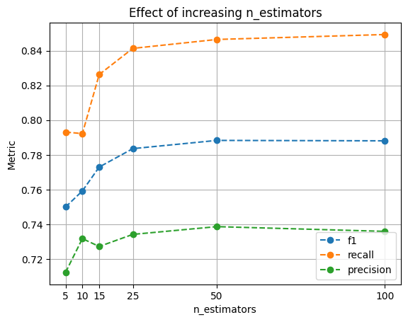
We can see that the increase in performance diminishes rapidly, after 50 estimators, there isn’t much performance gain. This analysis allows us to find these type of insights and focus on other parameters for improving performance.
Finally, let’s group by model type and see how our models are doing on average:
df = tracker.query(
    """
SELECT
    json_extract(parameters, '$.params.model_name') as model_name,
    AVG(json_extract(parameters, '$.metrics.precision[1][0]')) as precision,
    AVG(json_extract(parameters, '$.metrics.recall[1][0]')) as recall,
    AVG(json_extract(parameters, '$.metrics.f1[1][0]')) as f1
FROM experiments
GROUP BY model_name
""",
    as_frame=True,
).set_index("model_name")

ax = plt.gca()
df.plot(kind="barh", ax=ax)
ax.grid()
Console output (1/1):
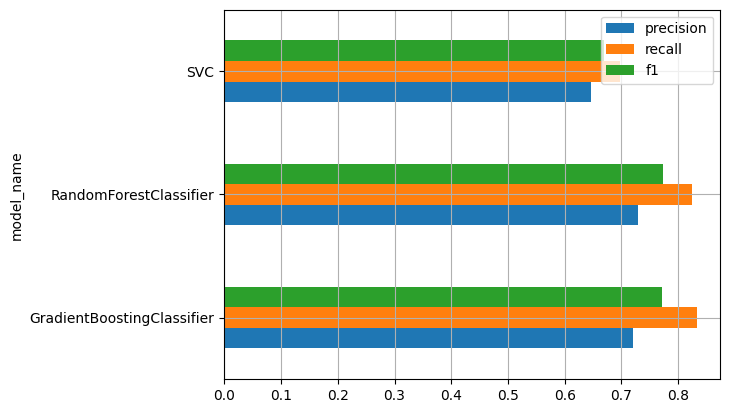
We see that Random Forest and Gradient Boosting have comparable performance, on average (although take into account that we ran more Random Forest experiments), and SVC has lower performance.
In this blog post, we showed how to export MLFlow data to a SQLite database, which allows us to use SQL to explore, aggregate and analyze our Machine Learning experiments, a lot better than MLFlow’s limited querying capabilities!
There are a few limitations to this first implementation, it’ll only work if you’re using the local filesystem for storing your MLFlow experiments and artifacts. And only .txt, .json and .png artifacts are supported. If you have any suggestions, feel free to open an issue on GitHub, or send us a message on Slack!
Seamless deployment for data scientists and developers. Ploomber handles infrastructure so you focus on building. Secure and scalable—from personal projects to enterprise apps. Support for Streamlit, Dash, Docker, and AI-powered applications. Because life's too short for deployment headaches.