Notebooks are great for rapid iterations and prototyping but quickly get messy. After working on a notebook, my code becomes difficult to manage and unsuitable for deployment. In production, code organization is essential for maintainability (it’s much easier to improve and debug organized code than a long, messy notebook).
In this post, I’ll describe how you can use our open-source tools to cover the entire life cycle of a Data Science project: starting from a messy notebook until you have that code running in production. Let’s get started!
The first step is to clean up our notebook with automated tools; then, we’ll automatically refactor our monolithic notebook into a modular pipeline with soorgeon; after that, we’ll test that our pipeline runs; and, finally, we’ll deploy our pipeline to Kubernetes. The main benefit of this workflow is that all steps are fully automated, so we can return to Jupyter, iterate (or fix bugs), and deploy again effortlessly.
Cleaning up the notebook

The interactivity of notebooks makes it simple to try out new ideas, but it also yields messy code. While exploring data, we often rush to write code without considering readability. Lucky for us, there are tools like isort and black which allow us to easily re-format our code to improve readability. Unfortunately, these tools only work with .py files; however, soorgeon enable us to run them on notebook files (.ipynb):
pip install soorgeon
soorgeon clean path/to/notebook.ipynb
Note: If you need an example notebook to try these commands, here’s one:
curl https://raw.githubusercontent.com/ploomber/soorgeon/main/examples/machine-learning/nb.ipynb -o notebook.ipynb
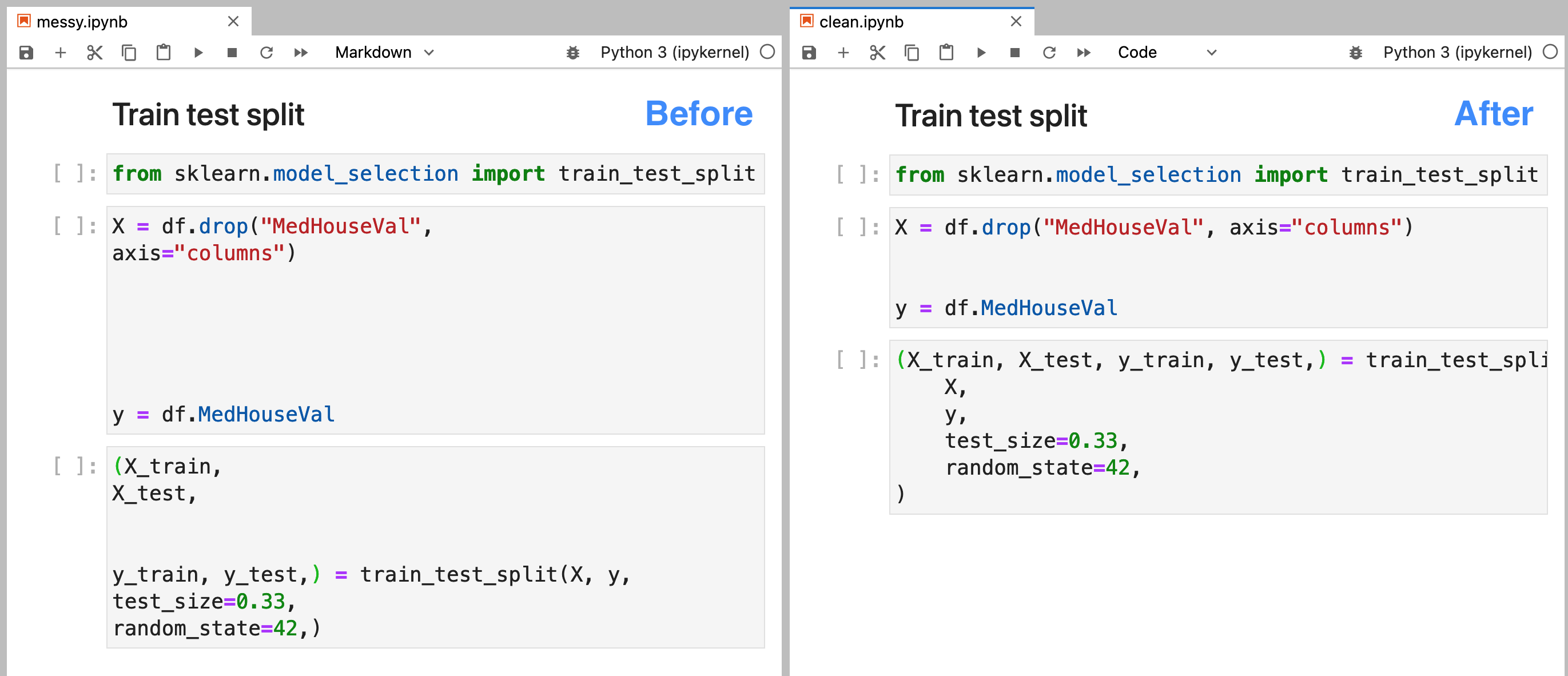
Check out the image at the beginning of this section: I introduced some extra whitespace on the left notebook. However, after applying soorgeon clean (picture on the right), we see that the extra whitespace went away. So now we can focus on writing code and apply soorgeon clean to use auto-formatting easily!
Refactoring the notebook
Creating analysis on a single notebook is convenient: we can move around sections and edit them easily; however, this has many drawbacks: it’s hard to collaborate and test. Organizing our analysis in multiple files will allow us to define clear boundaries so multiple pipelines can work in the project without getting into each other’s ways.
The process of going from a single notebook to a modular pipeline is time-consuming and error-prone; fortunately, soorgeon can do the heavy lifting for us:
pip install soorgeon
soorgeon refactor path/to/notebook.ipynb
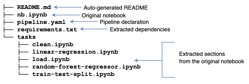
Upon refactoring, we’ll see a bunch of new files:

Ploomber turns our notebook into a modularized project automatically! It generates a README.md with basic instructions and a requirements.txt (extracting package names from import statements). Furthermore, it creates a tasks/ directory with a few .ipynb files; these files come from the original notebook sections separated by markdown headings. soorgeon refactor figures out which sections depend on which ones.
If you prefer to export .py files; you can pass the --file-format option:
soorgeon refactor nb.ipynb --file-format py
The tasks/ directory will have .py files this time:
.
├── README.md
├── nb.ipynb
├── pipeline.yaml
├── requirements.txt
└── tasks
    ├── clean.py
    ├── linear-regression.py
    ├── load.py
    ├── random-forest-regressor.py
    └── train-test-split.py
soorgeon uses Markdown headings to determine how many output tasks to generate. In our case, there are five of them. Then, soorgeon analyzes the code to resolve the dependencies among sections and adds the necessary code to pass outputs to the each task.
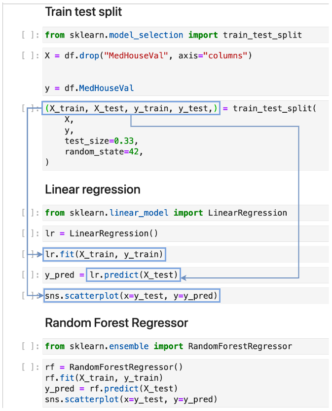
For example, our “Train test split” section creates a variables X, y, X_train, X_test, y_train, and y_test; and the last four variables are used by the “Linear regression” section:

By determining input and output variables, soorgeon determines that the “Linear regression” section depends on the “Train test split” section. Furthermore, the “Random Forest Regressor” section also depends on the “Train test split” since it also uses the variables generated by the “Train test split” section. With this information, soorgeon builds the dependency graph.
Testing our pipeline
Now it’s time to ensure that our modular pipeline runs correctly. To do so, we’ll use the second package in our toolbox: ploomber. Ploomber allows us to develop and execute our pipelines locally.
# install dependencies
pip install -r requirements.txt

# execute pipeline
ploomber build
name               Ran?      Elapsed (s)    Percentage
-----------------  ------  -------------  ------------
load               True         14.4272       38.6993
clean              True          7.89353      21.1734
train-test-split   True          2.98341       8.00263
linear-regression  True          3.77029      10.1133
random-forest-     True          8.20591      22.0113
ploomber offers a lot of tools to manage our pipeline; for example, we can generate a plot:
ploomber plot

We can see the dependency graph; there are three serial tasks: load, clean, and train-test-split. After them, we see two independent tasks: linear-regression, and random-forest-regressor. The advantage of modularizing our work is that members of our team can work independently, we can test tasks in isolation, and run independent tasks in parallel. With ploomber we can keep developing the pipeline with Jupyter until we’re ready to deploy!
Deployment
To keep things simple, you may deploy your Ploomber pipeline with cron, and run ploomber build on a schedule. However, in some cases, you may want to leverage existing infrastructure. We got you covered! With soopervisor, you can export your pipeline to Airflow, AWS Batch, Kubernetes, SLURM, or Kubeflow.
# add a target environment named 'argo'
soopervisor add argo --backend argo-workflows

# generate argo yaml spec
soopervisor export argo --skip-tests  --ignore-git

# submit workflow
argo submit -n argo argo/argo.yaml
soopervisor add adds some files to our project, like a preconfigured Dockerfile (which we can modify if we want to). On the other hand soopervisor export takes our existing pipeline and exports it to Argo Workflows so we can run it on Kubernetes.
By changing the --backend argument in the soopervisor add command, you can switch to other supported platforms.
Final remarks
Notebook cleaning and refactoring are time-consuming and error-prone, and we are developing tools to make this process a breeze. In this blog post, we went from having a monolithic notebook until we had a modular pipeline running in production—all of that in an automated way using open-source tools. So please let us know what features you’d like to see. Join our community and share your thoughts!


