


PostgreSQL is a popular relational database and is known for its reliability and advanced features. Now, imagine you have a Postgres database and want to create a Shiny application from the data. We can just query data from the database into a dataframe, and plot the data right? Well yes, we could. But what if we want to visualize many different subsets of data from the database? What if we want to show data from different tables in the Database? We would need a separate query for each of those things, and it could get really tedious.
However, by using Rpostgres, we can create a Shiny application that can interact directly with the database. Now, we can create a dropdown that allows the user to select which table in the database they want to visualize. We could create widgets that allow for advanced filtering. We can even create an interface for the users to write and execute their own queries on the app. Connecting Postgres to Shiny offers a powerful data visualization framework for all your data needs.
In this blog post, we will create a PostgreSQL database, upload data to the database, connect the database to an R Shiny application using Rpostgres, and deploy the application onto the Ploomber Cloud.
If you already have a PostgreSQL database set up, feel free to skip these steps.
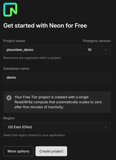
For the purpose of this blog, we can create a PostgreSQL database using Neon. Neon is a serverless Postgres database platform that allows developers to create a database in just a few clicks. A free tier with 0.5 GB of storage is available. After creating an account, you should be prompted to create a project. Enter the project name, the Postgres version you want, the database name, and your region.
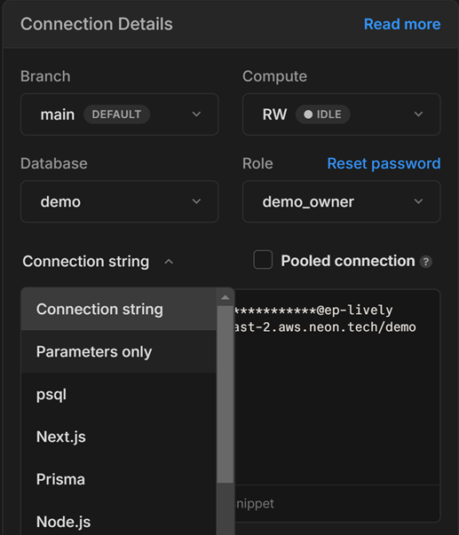
After creating the project, you should be redirected to your project dashboard. Under connection details, switch Connection string to Parameters only. We will need this information to connect to our database later.
If there is already data stored in your database, please skip this step.
For this blog, we will be using a public student performance data from two Portuguese schools. The dataset contains two csv files, student-mat.csv and student-por.csv, corresponding to students in a math class and Portuguese class, respectively. The tables share the same features, which include student age, absences, familial circumstances such as parent education level, and other personal information. The dataset is available for download here. We will be using this dataset to create a basic Shiny App for EDA.
To upload data to the database we just created, we can use Rpostgres, an open-source R package which offers a DBI compliant interface for Postgres in R. Uploading data using Rpostgres is simple, just follow these steps!
install.packages("RPostgres")
install.packages("DBI")
upload.R.This file will contain all the code for uploading data to our database. Make sure this file is separate from your shiny app as we do not want to perform any unintended modifications to our database. We will be running this file locally.
To establish a connection to the database, we can use the dbConnect function and pass in the database’s parameters. In your upload.R file, include the following code. Replace the specified fields using the parameters from your unique database. After running this script, you should see the connection to your database printed out.
library(DBI)

db <- "[DATABASE NAME]"
db_host <- "[YOUR HOST ADDRESS]"
db_port <- "[PORT NUMBER]" # You can use 5432 by default
db_user <- "[DATABASE USERNAME]"
db_pass <- "[DATABASE PASSWORD]"

conn <- dbConnect(
  RPostgres::Postgres(),
  dbname = db,
  host = db_host,
  port = db_port,
  user = db_user,
  password = db_pass
)

print(conn)
In upload.R, add code to read in whatever data you want to upload. Then, use the dbWriteTable function to upload a table to your database. Here, we read in two dataframes and uploaded two tables onto our database called math and portuguese.
math <- read.csv("data/student-mat.csv", sep=';')
por <- read.csv("data/student-por.csv", sep=';')

dbWriteTable(conn, name = "math", value = math)
dbWriteTable(conn, name = "portuguese", value = por)

dbListTables(conn)
Now, our database should contain those two tables. To verify the tables were uploaded, we can use dbListTables to print out a list of the tables in the database.
Now that the data is stored in the database, we can execute custom SQL queries in our R script using dbGetQuery!
query <- sprintf("SELECT * FROM math LIMIT 5")
df <- dbGetQuery(conn, query)
Lastly, it is always good practice to close the connection to your database once you are done interacting with it. Add the following code to the end of your upload.R file.
dbDisconnect(conn)
After we have our database setup, we can now use it alongside our shiny app! To do this, first establish a connection with the database as we have done above. In your app.R file, add the following code.
library(shiny)
library(DBI)
library(bslib)
library(dplyr)
library(ggplot2)

db <- "[DATABASE NAME]"
db_host <- "[YOUR HOST ADDRESS]"
db_port <- "[PORT NUMBER]"
db_user <- "[DATABASE USERNAME]"
db_pass <- "[DATABASE PASSWORD]"

conn <- dbConnect(
  RPostgres::Postgres(),
  dbname = db,
  host = db_host,
  port = db_port,
  user = db_user,
  password = db_pass
)

tables <- dbListTables(conn)
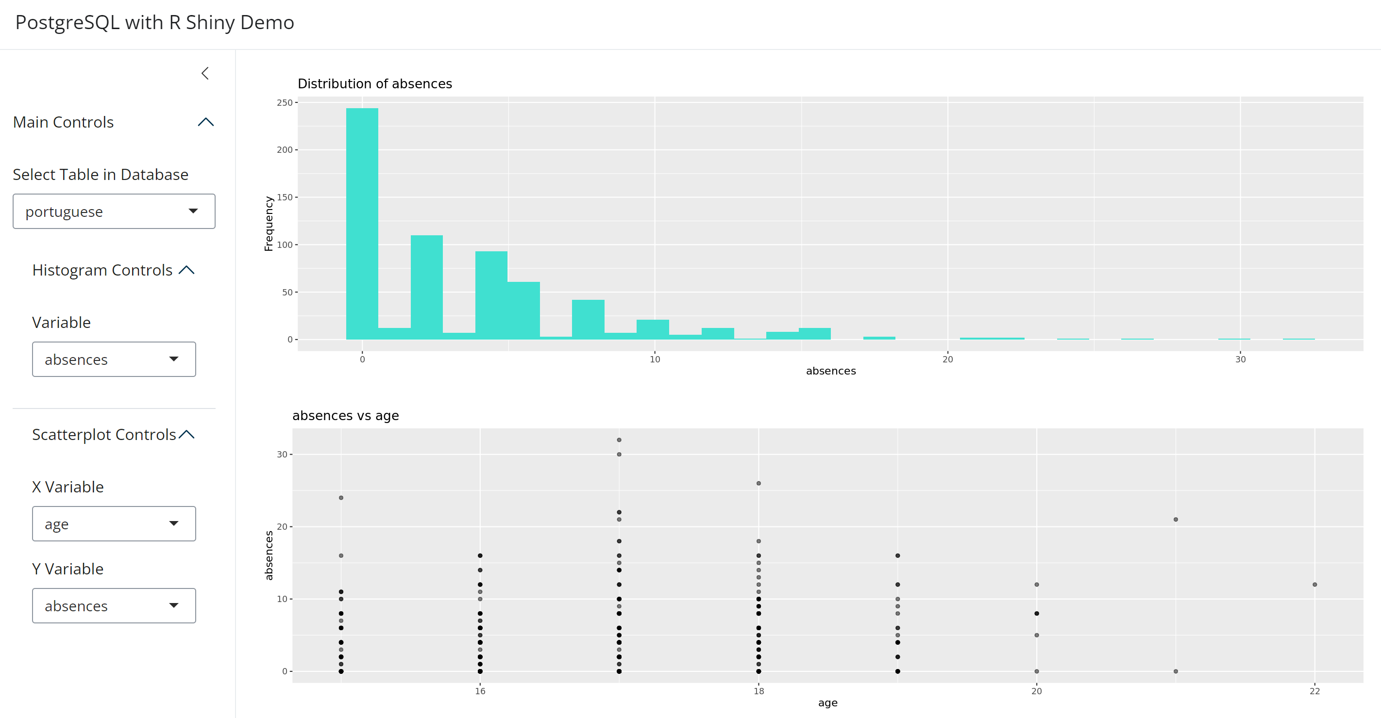
Next, we have some standard Shiny code to create an interactive UI. Since we integrated the app with our Postgres database, we are able to define a dropdown menu that allows the user to select which table in the database they want to visualize.
ui <- page_sidebar(
  title = "PostgreSQL with R Shiny Demo",

  sidebar = sidebar(
    accordion(
      accordion_panel(
        "Main Controls",
        # Allows user to select what table in the database they want to visualize.
        selectInput(inputId = "table",
          label = "Select Table in Database",
          choices = tables,
          selected = tables[]),
          accordion_panel(
            "Histogram Controls",
            selectInput(inputId = "hist_x",
              label = "Variable",
              choices = NULL)
          ),
          accordion_panel(
            "Scatterplot Controls",
            selectInput(inputId = "scatter_x",
              label = "X Variable",
              choices = NULL),
            selectInput(inputId = "scatter_y",
              label = "Y Variable",
              choices = NULL)
          )
      )
    )
  ),
  plotOutput(outputId = "hist"),
  plotOutput(outputId = "scatter")
)
In our server function, we use reactive values so that every time we select a different table in the database, we query from the new table, which then changes what options are available in the UI. In each of the plots, we use an SQL query to fetch data from the database. This means that we can write whatever query we want and display the result in whatever graph we need. For further details about reactive values check out the Shiny documentation.
server <- function(input, output, session) {
  quant_vars <- reactive({
    query <- sprintf("SELECT * FROM %s LIMIT 1", input$table)
    df <- dbGetQuery(conn, query)
    names(dplyr::select_if(df, is.numeric))
  })

  observe({
    updateSelectInput(session, "hist_x", choices = quant_vars())
    updateSelectInput(session, "scatter_x", choices = quant_vars())
    updateSelectInput(session, "scatter_y", choices = quant_vars())
  })

  output$hist <- renderPlot({
    query <- sprintf("SELECT * FROM %s", input$table)
    df <- dbGetQuery(conn, query)

    ggplot(df, aes_string(x = input$hist_x)) +
      geom_histogram(fill = "turquoise") +
      labs(title = sprintf("Distribution of %s", input$hist_x),
            x = input$hist_x,
            y = "Frequency")
  })

  output$scatter <- renderPlot({
    query <- sprintf("SELECT * FROM %s", input$table)
    df <- dbGetQuery(conn, query)

    ggplot(df, aes_string(x = input$scatter_x, y = input$scatter_y)) +
      geom_point(alpha = 0.5) +
      labs(title = sprintf("%s vs %s", input$scatter_y, input$scatter_x),
            x = input$scatter_x,
            y = input$scatter_y)
  })
}

shinyApp(ui = ui, server = server)
A screenshot of the shiny app is shown here. To run it yourself, visit this repository.
We will be using the Docker option to deploy to Ploomber Cloud. First, create a Ploomber Cloud account if you have not done so. The Docker deployment is available to professional but a 10-day free trial is available. To deploy the app, we just need to upload a .zip file containing the following files:
Here is a template for the Dockerfile, you may need to install additional dependencies depending on what R packages you might be using.
FROM rocker/shiny

WORKDIR /app

RUN apt-get update
RUN apt-get install -y libpq-dev

COPY install.R /app/

RUN Rscript install.R

COPY . /app

ENTRYPOINT ["Rscript", "startApp.R"]
The startApp.R file specifies which port and server the app will be run on. You can use this as the default.
library(shiny)
options(shiny.host = '0.0.0.0')
options(shiny.port = 80)
runApp('app.R')
The install.R file should contain all the packages that are used in the Shiny application.
install.packages("shiny")
install.packages("RPostgres")
install.packages("DBI")
install.packages("bslib")
install.packages("dplyr")
install.packages("ggplot2")
Now that you have your zip file prepared and you are logged into Ploomber Cloud, you should see this screen:
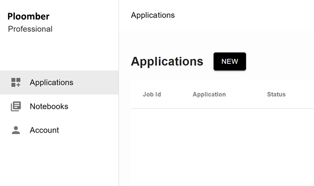
Click on NEW and under Overview, give your app a custom name and description.
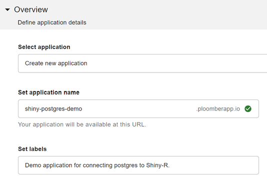
Once you are ready, select Docker under Framework and upload your zip file.
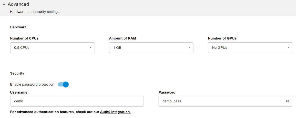
Next, you can optionally customize the hardware, such as the amount of RAM you want to run your application on. You could also enable password protection if you would like.
After you are done customizing, click create and the website will automatically deploy. Once it is deployed, you will be able to access the url. For further information on the deployment process, check out the Docker deployment documentation here.
And there we go! We now have a Shiny application that is connected to a Postgres database deployed on the Ploomber Cloud.
Seamless deployment for data scientists and developers. Ploomber handles infrastructure so you focus on building. Secure and scalable—from personal projects to enterprise apps. Support for Streamlit, Dash, Docker, and AI-powered applications. Because life's too short for deployment headaches.