


When it comes to interacting with SQL and integrating it with Python and the Jupyter Ecosystem, there are key considerations to keep in mind:
In this blog we will discuss methods for storing database credentials securely, and will share open source tools in the Jupyter and Python ecosystems to ease interacting with your database.
A fundamental principle in working with databases is the secure handling of your credentials. It is crucial to avoid hard-coding credentials into your scripts or notebooks. Here are some best practices to securely store and access your credentials:
keyring is a Python package that allows secure storage of passwords and API keys. You can use it to save your credentials and retrieve them securely within your script or notebook.
First, install the keyring library using pip:
%pip install keyring --quiet
Once installed, you can use the set_password method to save your credentials:
import keyring

# Setting up a keyring
service_id = "my_database"
user_id = "my_username"
password = "my_password"

keyring.set_password(service_id, user_id, password)
This will securely store your password for the given service_id and user_id.
Later, you can retrieve the password in your script or notebook like so:
import keyring

# Recovering password from the keyring
service_id = "my_database"
user_id = "my_username"

password = keyring.get_password(service_id, user_id)

# Now you can use these variables to connect to your database
By using keyring, you can ensure that your credentials are stored securely and are not exposed in your code or your environment variables. It’s a very useful tool when working with sensitive data in Python.
Another approach is to store credentials in a separate configuration file, which can be read by your script or notebook. Just ensure that this file is included in your .gitignore file so it doesn’t get uploaded to your version control system.
The configparser library in Python provides a straightforward interface for reading these files. Here’s how you can use it:
First, create a configuration file (let’s call it config.ini). Structure it like this:
[my_database]
user_id = my_username
password = my_password
Save and close config.ini. Make sure to add config.ini to your .gitignore file to prevent it from being tracked by Git.
Now you can use the configparser library in Python to read this file and retrieve your credentials:
import configparser

# Create a config parser
config = configparser.ConfigParser()

# Read the config file
config.read('config.ini')

# Retrieve your credentials
user_id = config.get('my_database', 'user_id')
password = config.get('my_database', 'password')

# Now you can use these variables to connect to your database
By using this method, you can keep your credentials separate from your code and out of your version control system, adding an extra layer of security.
One common practice is to store your credentials as environment variables. This method ensures that your credentials aren’t exposed in your code.
On Unix/Linux you can use the export command:
export DB_USER="your_username"
export DB_PASS="your_password"
On Windows, you can use the set command:
set DB_USER="your_username"
set DB_PASS="your_password"
These commands will set the environment variables for your current session. If you want to set them permanently, you will have to add them to your system’s environment variables, or include the export commands in your shell’s configuration file (like ~/.bashrc or ~/.bash_profile for bash on Unix/Linux/MacOS).
Once the environment variables are set, you can access them in your Python scripts or Jupyter notebooks using the os module:
import os

db_user = os.getenv("DB_USER")
db_pass = os.getenv("DB_PASS")

# Now you can use these variables to connect to your database
The os.getenv() function will return None if the environment variable is not set. If you want to ensure that your script stops with an error message when the environment variable is not set, you can use os.environ[] instead:
import os

try:
    db_user = os.environ["DB_USER"]
    db_pass = os.environ["DB_PASS"]
except KeyError:
    raise Exception("Required environment variables DB_USER and DB_PASS not set")

# Now you can use these variables to connect to your database
Remember that these environment variables are only accessible from within the same process (or its children) that set them. This means if you set an environment variable in a Jupyter notebook, it won’t be available in a different notebook or your Python script running in a different terminal.
Jupyter notebooks are fantastic for exploratory data analysis, rapid prototyping, and creating interactive data science documents. They allow you to write code, add comments, and visualize data all in one place, making them a preferred choice for data scientists.
Jupyter magics, such as Jupysql, can further enhance your SQL workflow. With Jupysql, you can run SQL queries directly in your notebook and load the results into a pandas dataframe. This can be especially helpful for ad-hoc queries or exploratory analysis where you need to quickly view and manipulate the data. It’s also convenient for demonstrating data extraction and transformation steps in a presentation or tutorial context.
Combining Jupyter notebooks with tools such as Voila can furthermore allow you to deploy your work as interactive dashboards.
Let’s begin by installing the jupysql library.
%pip install jupysql pandas openpyxl --quiet
We can create a sqlite instance and save it into a variable engine.
from sqlalchemy.engine import create_engine
# Create a SQL database
engine = create_engine("sqlite://")
We then load the extension and call our sqlite instance through the engine variable.
%load_ext sql
%sql engine
from IPython.display import display, Markdown
import requests
import pandas as pd
import io
import zipfile

url = "https://archive.ics.uci.edu/ml/machine-learning-databases/00445/Absenteeism_at_work_AAA.zip"

# Extract data from the zip file
response = requests.get(url)
zf = zipfile.ZipFile(io.BytesIO(response.content))

# Read the data into a pandas dataframe
df = pd.read_csv(zf.open("Absenteeism_at_work.csv"), sep=";", index_col=0)

# Rename columns to be more SQL friendly
df.columns = [c.replace(" ", "_").replace("/","_per_")for c in df.columns]

# turn all columns to lowercase
df.columns = [c.lower() for c in df.columns]


# Write the dataframe to the database
df.to_sql("absenteeism", engine, if_exists='replace')
Console output (1/1):
740
Make queries to the database.
%%sql
SELECT reason_for_absence,month_of_absence, day_of_the_week, seasons, service_time, age
FROM absenteeism
LIMIT 5
Console output (1/2):
*  sqlite://
Done.
Console output (2/2):
| reason_for_absence | month_of_absence | day_of_the_week | seasons | service_time | age |
|---|---|---|---|---|---|
| 26 | 7 | 3 | 1 | 13 | 33 |
| 0 | 7 | 3 | 1 | 18 | 50 |
| 23 | 7 | 4 | 1 | 18 | 38 |
| 7 | 7 | 5 | 1 | 14 | 39 |
| 23 | 7 | 5 | 1 | 13 | 33 |
We can save the query using the --save option followed by a query name.
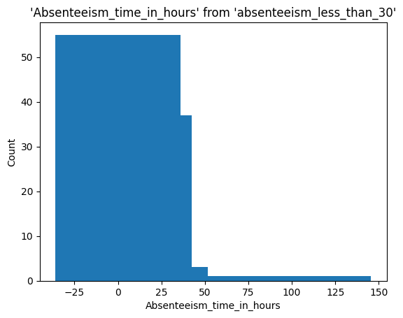
In the case below, we want to extract entries for employees younger than 30 years old.
%%sql --save absenteeism_less_than_30 --no-execute
SELECT * FROM absenteeism
WHERE Age < 30
Console output (1/1):
*  sqlite://
Skipping execution...
Let’s take a look at the distribution of absenteeism by day of the week using the %sqlplot magic
%sqlplot histogram \
    --with absenteeism_less_than_30 \
    --table absenteeism_less_than_30 \
    --column Absenteeism_time_in_hours
Console output (1/2):
<Axes: title={'center': "'Absenteeism_time_in_hours' from 'absenteeism_less_than_30'"}, xlabel='Absenteeism_time_in_hours', ylabel='Count'>
Console output (2/2):
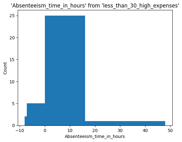
We can narrow down the data by saving it and selecting, for example, only those rows with a transportation expense greater than 300
%%sql --with absenteeism_less_than_30 --save less_than_30_high_expenses --no-execute
SELECT * FROM absenteeism_less_than_30
WHERE transportation_expense > 300
Console output (1/1):
*  sqlite://
Skipping execution...
%sqlplot histogram \
    --with less_than_30_high_expenses \
    --table less_than_30_high_expenses \
    --column Absenteeism_time_in_hours
Console output (1/2):
<Axes: title={'center': "'Absenteeism_time_in_hours' from 'less_than_30_high_expenses'"}, xlabel='Absenteeism_time_in_hours', ylabel='Count'>
Console output (2/2):
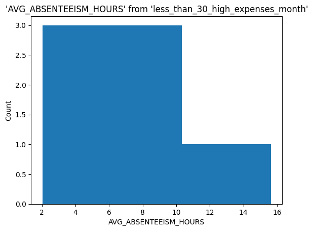
Group results by month and doing more complex queries
%%sql --with less_than_30_high_expenses --save less_than_30_high_expenses_month --no-execute
SELECT Month_of_absence, SUM(Work_load_Average_per_day_)  as TOTAL_LOAD_AVERAGE_PER_MONTH, SUM(Transportation_expense) as TOTAL_TRANSPORTATION_EXPENSE, AVG(Absenteeism_time_in_hours) as AVG_ABSENTEEISM_HOURS
FROM less_than_30_high_expenses
GROUP BY Month_of_absence
Console output (1/1):
*  sqlite://
Skipping execution...
Generate visualizations from via ggplot. Let’s understand the distribution for absenteeism for different days of the week.
%sqlplot histogram \
    --with less_than_30_high_expenses_month \
    --table less_than_30_high_expenses_month \
    --column AVG_ABSENTEEISM_HOURS
Console output (1/2):
<Axes: title={'center': "'AVG_ABSENTEEISM_HOURS' from 'less_than_30_high_expenses_month'"}, xlabel='AVG_ABSENTEEISM_HOURS', ylabel='Count'>
Console output (2/2):
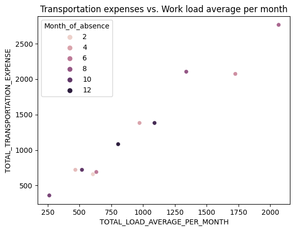
Visualizing using seaborn.
We can transform back the query to dataframe object and visualize.
import seaborn as sns
import matplotlib.pyplot as plt

result = %sql --with less_than_30_high_expenses_month SELECT * FROM less_than_30_high_expenses_month

result_df = result.DataFrame()


result_df.head()
Console output (1/2):
*  sqlite://
Done.
Console output (2/2):
| Month_of_absence | TOTAL_LOAD_AVERAGE_PER_MONTH | TOTAL_TRANSPORTATION_EXPENSE | AVG_ABSENTEEISM_HOURS | |
|---|---|---|---|---|
| 0 | 2 | 605.170 | 660 | 4.5 |
| 1 | 3 | 466.583 | 722 | 8.0 |
| 2 | 4 | 971.394 | 1382 | 5.5 |
| 3 | 5 | 1725.228 | 2073 | 5.5 |
| 4 | 6 | 631.507 | 691 | 4.5 |
sns.scatterplot(data=result_df, hue="Month_of_absence", x= "TOTAL_LOAD_AVERAGE_PER_MONTH", y="TOTAL_TRANSPORTATION_EXPENSE")
plt.title("Transportation expenses vs. Work load average per month")
plt.show()
Console output (1/1):
While Jupyter notebooks are great for exploration and visualization, IDEs shine when it comes to developing larger scripts, applications, or packages. They provide more robust code editing, debugging, and testing tools, making them better suited for production-level code or complex projects.
If you find yourself frequently reusing a particular SQL query or set of queries, it might be time to move that code from your notebook into a script or function within an IDE. This allows for better version control and easier maintenance. Likewise, if your notebook is becoming lengthy and difficult to navigate, consider transitioning to an IDE.
Here is a sample utils.py script you can reuse.
import sqlite3
import pandas as pd

def create_connection(db_path):
    """
    Creates a connection to the SQLite database specified by the db_path.
    :param db_path: The path to the SQLite database file.
    :return: The connection object or None if an error occurs.
    """
    try:
        conn = sqlite3.connect(db_path)
        return conn
    except sqlite3.Error as e:
        print(e)
    return None

def execute_query(conn, query):
    """
    Executes the given SQL query using the provided connection.
    :param conn: The connection object to the SQLite database.
    :param query: The SQL query string to execute.
    :return: The cursor object after executing the query.
    """
    try:
        cursor = conn.cursor()
        cursor.execute(query)
        return cursor
    except sqlite3.Error as e:
        print(e)
    return None

def load_results_as_dataframe(cursor):
    """
    Loads the results from a cursor object into a pandas DataFrame.
    :param cursor: The cursor object containing the query results.
    :return: A pandas DataFrame containing the query results.
    """
    columns = [description[0] for description in cursor.description]
    return pd.DataFrame(cursor.fetchall(), columns=columns)

def close_connection(conn):
    """
    Closes the connection to the SQLite database.
    :param conn: The connection object to the SQLite database.
    """
    conn.close()
You can then use the utils.py script as follows.
from utils import create_connection, execute_query, load_results_as_dataframe, close_connection

# Replace 'your_database.db' with the path to your SQLite database file
db_path = 'your_database.db'
query = "SELECT * FROM your_table_name;"

# Create a connection to the SQLite database
conn = create_connection(db_path)

if conn is not None:
    # Execute the query and load the results into a pandas DataFrame
    cursor = execute_query(conn, query)
    df = load_results_as_dataframe(cursor)

    # Close the connection to the SQLite database
    close_connection(conn)

    # Display the results in the DataFrame
    print(df)
else:
    print("Unable to connect to the database.")
The key to a successful SQL workflow is not to choose between Jupyter notebooks and IDEs, but to understand how to leverage the strengths of both.
Use Jupyter notebooks for initial data exploration, ad-hoc queries, and presenting your findings. Then, transition reusable queries, complex data transformations, or production-level code to an IDE for better maintainability and version control. This approach allows you to make the most of the interactivity and simplicity of notebooks, while also benefiting from the robust tools provided by IDEs.
In conclusion, the choice between Jupyter notebooks and IDEs, or a combination of the two, will depend on the requirements of your task and your personal workflow preferences. The most important thing is to ensure you’re using these tools securely and effectively to produce high-quality, reproducible data analyses. Happy coding!
This post was inspired by the discussion on this thread and includes code snippets generated by the community using ChatGPT
Seamless deployment for data scientists and developers. Ploomber handles infrastructure so you focus on building. Secure and scalable—from personal projects to enterprise apps. Support for Streamlit, Dash, Docker, and AI-powered applications. Because life's too short for deployment headaches.