


Existing experiment trackers come with a high setup cost. To get one working, you usually have to spin up a database and run a web application. After trying multiple options, I thought that using Jupyter notebooks could be an excellent choice to store experiment results and retrieve them for comparison. This post explains how I use .ipynb files to track experiments without any extra infrastructure.
Machine Learning is a highly iterative process: you don’t know in advance what combination of model, features, and hyperparameters will work best, so you need to make slight tweaks and evaluate performance. Experiment trackers help you log and manage all of your experiments.
However, most of them have a considerable maintenance cost: they usually require extra infrastructure such as a database and a web application to retrieve and compare experiments.
While paying this cost gives you many benefits, I’ve found that I rarely use an experiment tracker’s most advanced features. Furthermore, I only require to compare a few of my latest experiments and seldom care about an experiment I ran more than a few days ago, so I started using .ipynb files to log and compare experiments, greatly simplifying my workflow.
Jupyter notebooks (.ipynb) are JSON files. An empty notebook looks like this:
// sample .ipynb file (taken from nbformat documentation)
{
  "metadata" : {
    "kernel_info": {
        "name" : "the name of the kernel"
    },
    "language_info": {
        "name" : "the programming language of the kernel",
        "version": "the version of the language",
    }
  },
  "nbformat": 4,
  "nbformat_minor": 0,
  "cells" : [
      // list of cells (each one is a dictionary)
  ],
}
This pre-defined structure allows Jupyter to store code, output, and metadata in a single file. For our use case, let’s focus on the "cells" section:
"cells": [
    {
        "cell_type" : "code",
        "source" : "1 + 1",
    },
    // more cells...
]
"cells" contains a list of dictionaries (one per cell), where each element has a type (notebooks support different types of cells such as code or markdown) and other fields depending on its type. For example, code cells contain the source code ("source") and the associated output if the cell has executed:
"cells": [
    {
        "cell_type" : "code",
        "source" : "1 + 1",
        // cell's output
        "text": "2"
    },
    // more cells...
]
For brevity, I’m omitting details on the format specifics. However, if you’re curious, check out the nbformat package, which defines Jupyter notebook’s JSON schema.
.ipynb filesSince Jupyter notebooks have a pre-defined structure, we can parse them to extract data. For example, suppose you have trained a random forest and a neural network (random_forest.ipynb and nn.ipynb) to predict a continuous value, and you’re printing the mean square error in one of the cells:
// random_forest.ipynb
"cells": [
    // more cells...
    {
        "cell_type" : "code",
        "source" : "print(mse)",
        "text": "10.2"
    },
    // more cells...
]
// nn.ipynb
"cells": [
    // more cells...
    {
        "cell_type" : "code",
        "source" : "print(mse)",
        "text": "10.8"
    },
    // more cells...
]
You can load both files in a new notebook and extract the values for comparison:
from pathlib import Path
import json

rf = json.loads(Path('random_forest.ipynb').read_text())
svm = json.loads(Path('nn.ipynb').read_text())

# assume mean square error is the output of cell number 10
mse_rf = rf['cells'][10]['text']
mse_svm = svm['cells'][10]['text']

print(mse_rf)
print(mse_svm)
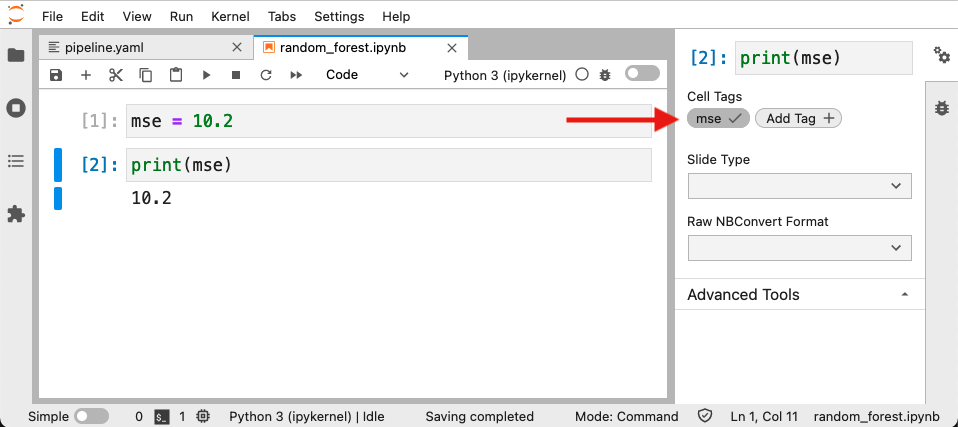
Accessing cells by an index number isn’t great; it’d be better to index them with some meaningful name. Fortunately, Jupyter notebook cells support tags. For example, to add a tag to a cell in JupyterLab 3.0+ (for details on tagging cells on earlier versions of JupyterLab or the Jupyter Notebook app, click here.):
Which translates into a .ipynb file that looks like this:
// random_forest.ipynb
"cells": [
    // more cells...
    {
        "tags": ["mse"],
        "cell_type": "code",
        "source" : "print(mse)",
        "text": "10.2"
    },
    // more cells...
]
We could access our accuracy metric with a bit more parsing logic by referring to the mse tag, but as we’ll see in an upcoming section, there’s a library that already implements this.
Extracting cells whose output is plain text is straightforward, but it’s limiting since we may want to compare cells whose output is a data frame or a chart. .ipynb files store tables as HTML strings, and images as base64 strings. The sklearn-evaluation package implements a notebook parser to extract and compare multiple types of outputs, all we need to do is tag our cells:
from sklearn_evaluation import NotebookIntrospector

nb = NotebookIntrospector('random_forest.ipynb')
# get the output of the cell tagged "mse"
nb['mse']
We can also load multiple notebooks at the same time:
from sklearn_evaluation import NotebookCollection

nbs = NotebookCollection(paths=['random_forest.ipynb', 'nn.ipynb'])

# compare mse between notebooks
nbs['mse']
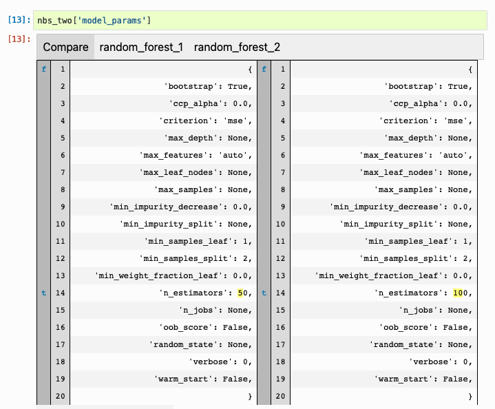
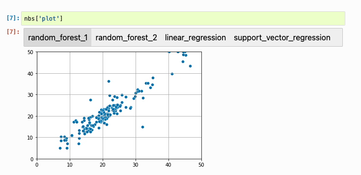
sklearn-evaluation automatically generates comparison views depending on the cell’s output. For example, if it’s a dictionary:
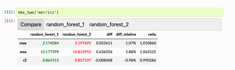
A table:
And a chart:
Using cell tags to identify outputs makes experiment tracking simple: no need to write any extra code. Instead, only print the result to retrieve, and tag the cell. For a complete example, click here.
sklearn-evaluation isn’t the only option. Scrapbook pioneered the idea of analyzing .ipynb files, the primary difference between them is that sklearn-evaluation uses cell tags, and scrapbook uses code to store data:
import scrapbook as sb

# store number
sb.glue("mse", 10.2)
And to retrieve the data:
nb = sb.read_notebook('random_forest.ipynb')
nb.scraps
papermillWe demonstrated how we could parse notebooks to retrieve their output. Let’s now discuss how to generate such notebooks. Since we want to compare multiple experiments, it makes sense to re-use the same code and only change its input parameters. papermill allows us to do that: we can create a notebook template, and execute it with different settings.
For example, say you have a train.ipynb notebook that looks like this:
# train.ipynb
from sklearn.model_selection import train_test_split
from sklearn_evaluation import plot

from my_project import load_training_data, instantiate_model

# default parameters
model_name = 'random_forest' # other values could be svm, neural_network, xgboost, etc
model_params = {'n_estimators': 10, 'max_depth': 5}

# load data
X, y = load_training_data()
X_train, X_test, y_train, y_test = train_test_split(X, y, test_size=0.20)

# instantiate the model using input parameters
model = instantiate_model(model_name, model_params)

# train
model.fit(X_train, y_train)

# predict
y_pred = model.predict(X_test)

# evaluate
plot.confusion_matrix(y_test, y_pred)
By default, the previous snippet trains a random forest. However, we can change model_name and model_params to switch to a different model. We may even define other parameters (e.g., select a feature subset, row subset, etc.) to customize our training notebook further. When using papermill , we can easily add a new cell to override default values:
# train.ipynb
# ...
# ...

# default parameters (what we typed)
model_name = 'random_forest' # other values could be svm, neural_network, xgboost, etc
model_params = {'n_estimators': 10, 'max_depth': 5}


# parameters injected by papermill (this overrides default parameters)
model_name = 'neural_network'
model_params = {'hidden_layer_sizes': [10, 10], 'activation': 'relu'}

# training code
# ...
# ...
Notebook parametrization allows us to use our template with different values and generate multiple notebook files using the same code. The following snippet shows how to run our experiments:
import papermill as pm

experiments = [
    {
        'model_name': 'random_forest',
        'model_params': {
            'n_estimators': 10,
            'max_depth': 5
        }
    },
    {
        'model_name': 'neural_network',
        'model_params': {
            'hidden_layer_sizes': [10, 10],
            'activation': 'relu'
        }
    },
    # more models to train...
]

for params in experiments:
    pm.execute_notebook(input_path='template.ipynb',
                        output_path=f'{exp["model_name"].ipynb}',
                        parameters=params)
When execution finishes, we’ll have:
random_forest.ipynbneural_network.ipynbAnd we can proceed to analyze the results with sklearn-evaluation or scrapbook.
Alternatively, we can use Ploomber, which allows us to create pipelines by writing a pipeline.yaml file. papermill’s example looks like this in Ploomber:
executor: parallel

tasks:
    - source: train.ipynb
      name: train-
      product: output/train.ipynb
      grid:
        # experiment 1: random forest
        - model_name: random_forest
          model_params:
            n_estimators: 10
            max_depth: 5
        # experiment 2: neural network
        - model_name: neural_network
          model_params:
            hidden_layer_sizes: [10, 10]
            activation: relu
        # more models to train...
To run all the experiments, we execute the following in the terminal:
ploomber build
Using Ploomber has many benefits: it runs notebooks in parallel; it allows us to use scripts as an input format (i.e., source: train.py), performing the conversion and execution to .ipynb for us; and even running notebooks in the cloud!
I’m working on a project where we make frequent improvements to a model that’s in production. Although our testing suite automatically checks candidate models' performance, we still review metrics manually since we may detect errors not yet implemented in our testing suite. Whenever we have a candidate model, we compare it against the metrics of the model in production. Since each model experiment generates a .ipynb file with the same format, we load the two files (say candidate.ipynb, and production.ipynb) and generate an evaluation report using another notebook template. The code looks like this:
# model_comparison.ipynb
nbs = NotebookCollection(paths=['candidate.ipynb', 'production.ipynb'])

nbs['metrics_table']

nbs['plot_1']

nbs['plot_2']

# ...
The model comparison report allows us to contrast parameters, tables, and charts quickly; we can easily spot performance differences that are hard to detect with an automated test. For example, this report once saved us from deploying a model trained on corrupted data.
Experiment trackers come with a significant setup cost: installing a separate package, spinning up a database, and running a web application. And while they provide a lot of features, I’ve found that generating .ipynb files for each experiment and then comparing their outputs is all I need.
This approach doesn’t need any extra infrastructure; furthermore, it allows me to share my findings quickly and doesn’t require additional code to log experiments, making it a straightforward yet powerful approach for comparing Machine Learning experiments.
If you like my work, please consider showing your support with a star on GitHub. Also, if you have any questions, feel free to join our community and share them with us.