

Putting notebooks and production in the same sentence is a sure way to trigger a heated online debate. This topic comes up frequently, and it’s common to hear that teams completely dismiss notebooks because they’re not for production. Unfortunately, the discussion often centers on problems already fixed by current tools, but the solutions are still unknown for many practitioners. This post shows how to overcome some of Jupyter notebook’s limitations, proposes a workflow to streamline their use in production, and discusses problems that remain to be solved.
The origins of computational notebooks come from literate programming, introduced by Donald Knuth. At its core, this idea advocates for writing programs that interleave source code and documentation to make programs more readable. Notebooks extend this idea by adding other capabilities such as embedded graphics and interactive code execution.
Combining these three elements (interleaving code with documentation, embedded graphics, and interactivity) provides a powerful interface for data exploration. Real-world data always comes with peculiarities; interleaved documentation helps to point them out. Data patterns only surface when visualizing the data through embedded graphics. Finally, interactivity allows us to iterate on our analysis to avoid re-executing everything from scratch with every change.
Up until this point, I haven’t referred to any notebook implementation in particular. There are many flavors to choose from, but for the remainder of this post, I’ll refer to Jupyter notebooks.
To support interleaved documentation, Jupyter supports Markdown cells. For embedded graphics, Jupyter serializes images using base64, and for interactivity, it exposes a web application that lets users add and execute code.
Such implementation decisions have significant side effects:
.ipynb files are JSON files. git diff outputs an illegible comparison between versions, making code reviews difficult.The first two problems are consequences of the .ipynb implementation. Fortunately, they’re easily solvable with current tools. For example, if we are ok storing relatively big files on git, we can configure git to use a different algorithm to generate the diff view for .ipynb files, nbdime allows us to do that.
If we care about git versioning and file size, we can completely substitute the .ipynb format. Jupytext allows Jupyter to open .py (among others) files as notebooks; the caveat is that any output is lost since .py files do not support embedded graphics. However, you can use jupytext pairing feature to keep the output in a separate file.
Most people are unaware that Jupyter is agnostic to the underlying file format. Just because something feels like a notebook doesn’t mean it has to be a .ipynb file. Changing the underlying file format solves the size and versioning issues; let’s focus on the real problem: hidden state.
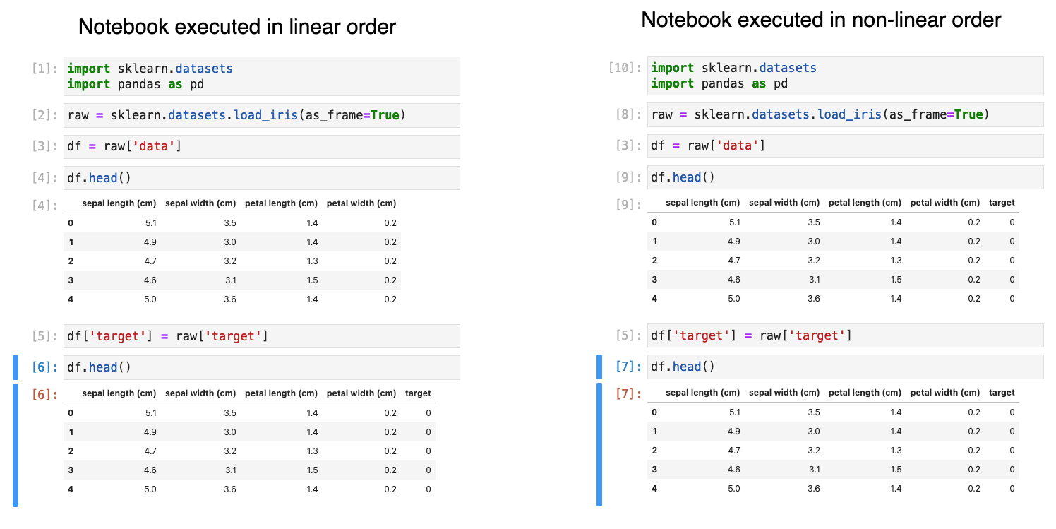
Jupyter allows users to add and execute code cells interactively. When working with a new dataset, this is extremely helpful. It enables us to explore and clean our data while keeping a record (code and output) of what we’ve executed so far. However, the data exploration process is mostly trial and error; we often modify and re-execute previous cells, causing the history of cells not to be linear. Recently, an analysis of 10 million notebooks on GitHub found out that 36% of Jupyter notebooks had cells that executed in a non-linear order.
Notebook’s hidden state is by far the most significant (and valid) criticism of notebooks. It’s the notebook’s paradox: arbitrary cell execution eases data exploration, but its over-use often produces broken irreproducible code.
But even perfectly linear notebooks have other problems; mainly, that they are hard to debug and test. There are two primary reasons for this. First, notebooks evolve organically, and once they grow large enough, there are too many variables involved that it’s hard to reason about the execution flow. The second reason is that functions defined inside the notebook cannot be unit tested (although this is changing) because we cannot easily import functions defined in a .ipynb file into a testing module. We may decide to define functions in a .py file and import them into the notebook to fix this. Still, when not done correctly, this results in manual editions to sys.path or PYTHONPATH that cause other problems.
Given such problems, it’s natural that teams disallow the use of notebooks in production code. A common practice is to use notebooks for prototyping and refactor the code into modules, functions, and scripts for deployment. Often, data scientists are in charge of prototyping models; then, engineers take over, clean up the code and deploy. Refactoring notebooks is a painful, slow, and error-prone process that creates friction and frustration for data scientists and engineers.
In a normal refactoring process, engineers would make small changes and run the test suite to ensure that everything is still working correctly. Unfortunately, it’s rarely the case that data scientist’s code comes with a comprehensive test suite (in data scientist’s defense: it’s hard to think about code testing when your work output is measured by how good your model is). Lack of tests dramatically increasing the difficulty of the refactoring process.
On the other hand, software projects require maintenance. While engineers may be able to do some of this, a data scientist is best suited for tasks such as model re-training. After the refactoring process occurs, even the data scientist who authored the original code will have difficulty navigating through the refactored version that engineers deployed. Even worse, since the code is not in a notebook anymore, they can no longer execute it interactively. What ends up happening is a lot of copy-pasting between production code and a new development notebook.
As you can see, this is an inefficient process that often leads to broken pipelines and drastically slows down the time required to deploy updates. All of this creates an excessive burden that, in some cases, causes companies to abandon Machine Learning projects due to the high maintenance costs.
For most of the Machine Learning projects I’ve done in my career, I’ve been responsible for the end-to-end process: exploring datasets to create new model features, train models, and deploy them. I’ve experienced first-hand this painful refactoring process where I have to move back and forth between a notebook environment and the production codebase. During my first years working with data, I took this problem for granted and learned to live with it. However, as I started taking part in more critical projects, stakes were too high for me to continue working this way, and I developed a workflow that has allowed me to overcome these challenges for the most part.
When designing this workflow, I’ve put simplicity first. Data science teams have to move fast because their work is inherently experimental. This approach isn’t a definitive solution, but it’s a massive improvement over current practices. There is a lot of room for innovation in notebooks and Machine Learning tooling to champion a workflow that gives data scientists the power of interactive development and, at the same time, allows them to better collaborate with engineering teams in the deployment process.
The proposed workflow is as follows:
git push.setup.py file).Let’s now discuss each one in detail.
As described earlier, the .ipynb format doesn’t play nicely with git. However, Jupyter’s architecture allows the use of alternative file formats. Jupytext enables users to open .py as notebooks, effectively fixing git versioning issues and facilitating code reviews. Data scientists can develop their code interactively from Jupyter, but the repository will only contain .py files. The rest of the article keeps using the term notebooks, but remember that we refer to Python scripts compatible with Jupyter.
These three problems are highly related and much more challenging to solve. As with any other software project, the solution lies in developing modularized and testable code. However, the challenge is how to apply it to a highly uncertain environment that requires fast iterations and employs Jupyter notebooks as its primary development tool.
We want to achieve the following:
Testing data processing code is challenging on its own because of runtime. We cannot afford to run all our processing code on every change because it may take hours to finish. Fortunately, we can detect the most common errors with small amounts of data: missing columns, wrong array shapes, incompatible data types, etc. Hence, an effective strategy is to run all notebooks with a data sample on every push to eliminate the chance of having broken notebooks. Nevertheless, since we are not testing the notebook’s output, this isn’t robust; but we can incorporate more complete tests as our project matures. If you want to learn more about testing Data Science pipelines, check out my talk at PyData 2020.
To automate notebook execution, we can use papermill or nbclient. Note that since we switched the underlying format, we’ll have to use jupytext to convert .py files back to .ipynb and then execute them.
Modularizing code is a regular practice in software engineering because it makes the code more testable and maintainable. Yet, it’s common for data scientists to code entire projects in a single notebook. Why? Convenience. Once you break down a project into multiple parts, you have to deal with technical difficulties that require extra work from a data scientist, and in some cases, such work goes beyond their area of expertise. Simplifying the modularization process is why (among many other reasons) dbt is thriving: it allowed data analysts to break down colossal SQL scripts into multiple parts assembled into one coherent pipeline. We can apply the same logic to notebooks.
Notebook modularization is where most tools fall short. While many workflow orchestrators support notebook execution, they do not make the process enjoyable. Helping data scientists (myself included) write more maintainable and modularized pipelines was my primary motivation to create Ploomber.
Ploomber allows data scientists to create a data pipeline from multiple notebooks in two steps:
pipeline.yaml file.For example, a typical pipeline.yaml looks like this:
tasks:
    - source: get-data.py
      product:
        nb: get-data.ipnyb
        data: data.csv

    - source: clean.py
      product:
        nb: clean.ipnyb
        data: clean.csv

    - source: fit-model.py
      product:
        nb: fit-model.ipnyb
        data: model.pickle
The .py scripts are recognized as “notebooks” by Jupyter, thanks to the Ploomber (and jupytext) plug-in; hence, data scientists can develop interactively. However, during execution, Ploomber converts them to .ipynb and executes them, allowing us to keep the source (.py) and output (tables and charts in the .ipynb file) separate. Furthermore, tasks can generate any other number of outputs, such as data files.
To establish the execution order, users only have to declare notebooks that must execute before the one we are working on. For example, to clean data, we must download the raw version, so we’ll do something like this in clean.py:
upstream = ['get-data']
That’s it. If we reload the notebook, we’ll see a new cell right below our list of dependencies:
# original cell (what I wrote)
upstream  = ['get-data']

# injected cell (what ploomber added)
upstream = {
    'get-data': {
      'data': 'data.csv'
    }
}
Ploomber parses our reference and adds a new variable that contains the location of our inputs. We can continue building this way and create pipelines with dozens of tasks without having to keep track of the output of each one. Since it’s simple to split logic across files, multiple people can work on it simultaneously. Ploomber helps create maintainable pipelines that feel like a single notebook.
By referencing other tasks with the upstream variable, we also determine execution order, allowing us to create a pipeline like this:
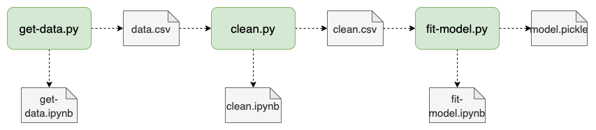
To execute the whole pipeline, we run: ploomber build.
Notebook modularization has many benefits: it allows us to run parts in isolation for debugging, add integration tests to check the integrity of each output, parametrize the pipeline to run with different configurations (development, staging, production), parallelize independent tasks, etc.
Code declared in a notebook cannot be easily imported from other notebooks, which causes a lot of copy-pasting among .ipynb files. As a result, when deploying a model, engineers often have to deal with project structures like this:
utils.py
plots.py
Untitled.ipynb
train.ipynb
train2.ipynb
features.ipynb
Refactoring a project like the one above is an authentic nightmare. When an engineer has to refactor such a project for deployment, it’s too late: notebooks may easily contain thousands of cells with several portions copy-pasted among them and no unit tests. Instead, we should aim to keep a minimum of code quality at all stages of the project.
First, the use of scripts as notebooks (as mentioned earlier) facilitates code reviews since we no longer have to deal with the complexities of diffing .ipynb files. Second, by providing data scientists a pre-configured project layout, we can help them better organize their work. For example, a better-organized project may look like this:
# data scientists can open these files as notebooks
tasks/
  get.py
  clean.py
  features.py
  train.py

# function definitions
src/
  get.py
  clean.py
  features.py
  train.py

# unit tests for code in src/
tests/
  clean.py
  features.py
  train.py
The previous example layout explicitly organizes a project in three parts. First, we replace .ipynb files with .py and put them in the tasks/ directory. Second, the logic required multiple times is abstracted in functions and stored under src/. Finally, functions defined in src/ are unit tested in tests/.
To ensure this layout works, the code defined in src/ must be importable from tasks/ and tests/. Unfortunately, this won’t work by default. If we open any of the “notebooks” in tasks/, we’ll be unable to import anything from src/ unless we modify sys.path or PYTHONPATH. Still, if a data scientist cannot get around the finickiness of the Python import system, they’ll be tempted to copy-paste code.
Fortunately, this is a simple problem to solve. Add a setup.py file for Python to recognize your project as a package, and you’ll be able to import functions from src/ anywhere in your project (even in Python interactive sessions). Whenever I share this trick with fellow data scientists, they start writing more reusable code. To learn more about Python packaging, click here.
Discussing the use of notebooks in productions is always an uphill battle. Most people take as undeniable truth that notebooks are just for prototyping but I don’t believe so. Notebooks are a fantastic tool for working with data, and while current tools are making it easier to use notebooks to write production-ready code, there is still a lot of work to do.
Part of that work is developing better tools that go beyond improving the notebook experience: there is undoubtedly a lot of value in providing features such as live collaboration, better integration with SQL, or managed Jupyter Lab in the cloud; however, notebooks will still be perceived as a prototyping tool if we don’t innovate in areas that are more important when deploying code such as orchestration, modularization, and testing.
Furthermore, part of the work is to dispel myths about how notebooks work. I want development practices in Data Science to take the best of notebooks and evolve, not dismiss them and go back to the same methods of the pre-notebook era.
If you’d like help adopting a workflow that embraces notebooks in production please reach out, I’m always happy to chat about these topics.
Special thanks to Alana Anderson and Sarah Krasnik for reading earlier drafts and providing invaluable feedback.
Seamless deployment for data scientists and developers. Ploomber handles infrastructure so you focus on building. Secure and scalable—from personal projects to enterprise apps. Support for Streamlit, Dash, Docker, and AI-powered applications. Because life's too short for deployment headaches.